Chromatic dispersion and its compensation

Standard single-mode fibre spreads a 32 GBd signal over many symbols: \(D = 17\) ps/(nm·km) accumulate 1360 ps/nm over 80 km, and the received 16-QAM constellation collapses into a cloud. Dispersion is an all-pass filter, \(e^{j \beta_2 \omega^2 L / 2}\), so the receiver undoes it exactly in the frequency domain (comnum.cdc()), or with an FIR whose length grows with the accumulated dispersion (comnum.cd_fir_taps()).

import matplotlib.pyplot as plt
import numpy as np

import comnum
from comnum.plot import BLUE, CRIMSON, GREY, LABEL, TEAL

RS, SPS = 32e9, 2
FS = RS * SPS
fiber = comnum.FiberParams(n_spans=1, span_km=80.0)
c = comnum.Constellation("qam", 16).normalized()
rng = comnum.Rng(4)
_, x = comnum.symbols(c, 8192, rng)
h = comnum.pulse_shape("rrc", SPS, n_taps=2 * 128 + 1, rolloff=0.1)
tx = comnum.fir_filter(h, comnum.upsample(x, SPS))
# the span loss is compensated by a noisy amplifier: an OSNR-limited link at 20 dB SNR
rx = comnum.awgn(
    comnum.linear_fiber_channel(tx, fiber, 80.0, FS), 20.0, rng, fs=FS, bandwidth_hz=RS
)


def symbols(r):
    return comnum.pnorm(comnum.downsample(comnum.fir_filter(h, r), SPS))[200:-200]


cases = {
    "back to back": comnum.awgn(tx, 20.0, rng, fs=FS, bandwidth_hz=RS),
    "80 km, no compensation": rx,
    "80 km, compensated": comnum.cdc(rx, fiber, 80.0, FS),
}
fig, axes = plt.subplots(1, 3, figsize=(9.5, 3.6), sharex=True, sharey=True)
for ax, (name, r) in zip(axes, cases.items(), strict=True):
    z = symbols(r)
    ber, _, snr = comnum.fast_ber_calc(z, x[200:-200], c)
    ax.scatter(z.real, z.imag, s=2, color=BLUE, alpha=0.35, linewidth=0)
    ax.set(title=name, aspect="equal", xlim=(-1.8, 1.8), ylim=(-1.8, 1.8))
    ax.text(
        0.03,
        0.03,
        f"SNR {snr:.1f} dB\nBER {ber:.1e}",
        transform=ax.transAxes,
        fontsize=8,
        color=LABEL,
        va="bottom",
    )
fig.tight_layout()

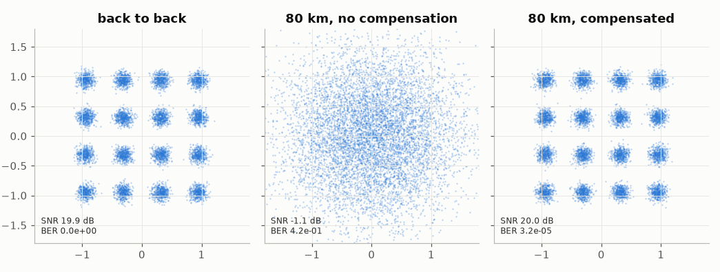
The FIR alternative: OptiCommPy’s length rule, and its accuracy against the exact compensation.

n = comnum.cd_taps_needed(fiber, 80.0, RS, FS)
taps = comnum.cd_fir_taps(fiber, 80.0, FS, max(n, 1) | 1)
z = symbols(comnum.convolve(taps, rx)[len(taps) // 2 : len(taps) // 2 + rx.size])
print(f"{n} taps for 80 km: SNR {comnum.fast_ber_calc(z, x[200:-200], c)[2]:.1f} dB")

48 taps for 80 km: SNR 19.9 dB

Optimal FIR filters in the least-squares sense

Savory’s filter (comnum.cd_savory_taps(); S. J. Savory, Opt. Express 16(2), 2008) truncates the impulse response of the analog compensation to \(N = 2\lfloor 2\pi K \rfloor + 1\) taps, with \(K = -\beta_2 L f_s^2 / 2\) (comnum.cd_dispersion_factor()). Eghbali, Johansson, Gustafsson and Savory (J. Lightw. Technol. 32(8), 2014) design the taps that minimise the energy of the error \(E = \frac{1}{2\pi}\int_{-\Omega}^{\Omega} |H(e^{j\omega}) - e^{jK\omega^2}|^2 d\omega\) (comnum.cd_ls_taps(), comnum.cd_ls_error()): over the whole band (\(\Omega = \pi\)) the taps are closed-form, and over the band of the signal (\(\Omega = \pi(1 + \rho)/L\) for a roll-off \(\rho\) at \(L\) samples per symbol) far fewer taps reach the same error. The example below is example 1 of the paper: 4000 km of fibre with \(D = 17\) ps/(nm·km), 10.7 GBd at two samples per symbol, roll-off 0.25, so \(K \approx 19.9\) and \(N = 251\).

The error of the least-squares filter falls with its length; Savory’s error is smallest at its own length and grows beyond (Sec. III-A2 of the paper); frequency sampling (comnum.cd_fir_taps()) fits the response only at \(N\) frequencies. The closed form of \(E\) loses its precision near \(10^{-16}\): the curves are clipped there.

FS1 = 21.4e9
SPAN = 4000.0
fib = comnum.FiberParams(d_ps_nm_km=17.0, fc_hz=3e8 / 1553e-9)
band = FS1 * 1.25 / 4
print(
    f"K = {comnum.cd_dispersion_factor(fib, SPAN, FS1):.2f}, N = {len(comnum.cd_savory_taps(fib, SPAN, FS1))}"
)


def err_db(taps, b=FS1 / 2):
    return comnum.lin2db(max(comnum.cd_ls_error(taps, fib, SPAN, FS1, band_hz=b), 1e-16))


lengths = np.arange(101, 352, 10)
curves = {
    "Savory, whole band": [
        err_db(comnum.cd_savory_taps(fib, SPAN, FS1, n_taps=n)) for n in lengths
    ],
    "frequency sampling, whole band": [
        err_db(comnum.cd_fir_taps(fib, SPAN, FS1, n)) for n in lengths
    ],
    "least squares, whole band": [err_db(comnum.cd_ls_taps(fib, SPAN, FS1, n)) for n in lengths],
    "least squares, band of the signal": [
        err_db(comnum.cd_ls_taps(fib, SPAN, FS1, n, band_hz=band, epsilon=1e-14), band)
        for n in lengths
    ],
}
fig, ax = plt.subplots(figsize=(6.4, 3.8))
for (name, e), color, marker in zip(
    curves.items(), [CRIMSON, GREY, BLUE, TEAL], "sdo^", strict=True
):
    ax.plot(lengths, e, marker=marker, color=color, markersize=4, label=name)
ax.axvline(251, color=GREY, linewidth=0.8, linestyle=":")
ax.set(xlabel="number of taps", ylabel="error energy E (dB)", ylim=(-165, 5))
ax.grid(alpha=0.3)
ax.legend(fontsize=8)
fig.tight_layout()

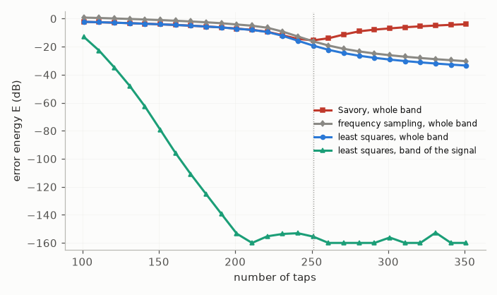
K = 19.91, N = 251

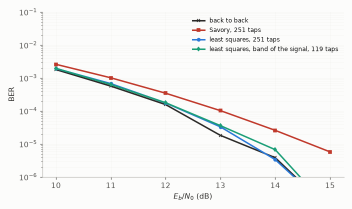
The BER of 16-QAM through the chain of Fig. 2 of the paper: ideal root-raised-cosine filters at both ends, the dispersion, white noise, the FIR, at \(E_b/N_0 = 10\) to 15 dB. The least-squares filter of 251 taps nearly reaches the back-to-back curve, Savory’s filter of the same length loses about 0.9 dB at \(10^{-5}\), and the band-limited filter matches the 251 taps of Savory with 119 (Figs. 5 and 9 of the paper; validation/tests/fiber/eghbali2014.rs checks these points).

NSYM = 1 << 19
g = comnum.rrc_spectrum(NSYM, 2, 0.25) * np.sqrt(2)
w = 2 * np.pi * np.fft.fftfreq(2 * NSYM)
k1 = comnum.cd_dispersion_factor(fib, SPAN, FS1)
c16 = comnum.Constellation("qam", 16).normalized()


def ber_16qam(taps, ebn0_db, rng):
    _, a = comnum.symbols(c16, NSYM, rng)
    u = np.zeros(2 * NSYM, complex)
    u[::2] = a
    k = 0.0 if taps is None else k1
    y = np.fft.ifft(np.fft.fft(u) * g * np.exp(-1j * k * w**2))
    y = y + rng.complex_noise(y.size, 1 / (4 * comnum.db2lin(ebn0_db)))
    yf = np.fft.fft(y) * g
    if taps is not None:
        h = np.zeros(y.size, complex)
        h[(np.arange(taps.size) - taps.size // 2) % y.size] = taps
        yf = yf * np.fft.fft(h)
    return comnum.fast_ber_calc(np.fft.ifft(yf)[::2], a, c16)[0]


ebn0 = np.arange(10.0, 15.5, 1.0)
filters = {
    "back to back": None,
    "Savory, 251 taps": comnum.cd_savory_taps(fib, SPAN, FS1),
    "least squares, 251 taps": comnum.cd_ls_taps(fib, SPAN, FS1, 251),
    "least squares, band of the signal, 119 taps": comnum.cd_ls_taps(
        fib, SPAN, FS1, 119, band_hz=band, epsilon=1e-14
    ),
}
rng = comnum.Rng(14)
fig, ax = plt.subplots(figsize=(6.4, 3.8))
for (name, taps), color, marker in zip(
    filters.items(), [LABEL, CRIMSON, BLUE, TEAL], "xsod", strict=True
):
    b = [ber_16qam(taps, e, rng) for e in ebn0]
    ax.semilogy(ebn0, np.maximum(b, 1e-7), marker=marker, color=color, markersize=4, label=name)
ax.set(xlabel="$E_b/N_0$ (dB)", ylabel="BER", ylim=(1e-6, 1e-1))
ax.grid(alpha=0.3, which="both")
ax.legend(fontsize=8)
fig.tight_layout()

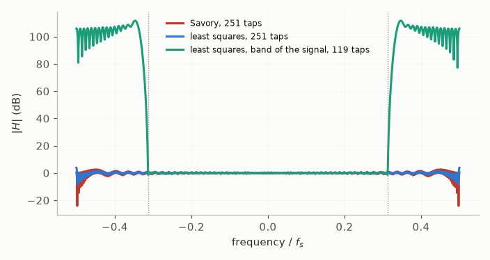
The price of the band-limited design: the response outside the band of the signal is not constrained and exceeds \(10^{5}\) (100 dB), so the receive filter must reject that band; the paper assumes ideal pulse-shaping filters. With a truncated root-raised-cosine filter of finite stopband, the amplified out-of-band noise ruins the link; a larger penalty \(\epsilon\) lowers this gain at the cost of a larger error in the band.

f = np.linspace(-0.5, 0.5, 2001)
fig, ax = plt.subplots(figsize=(6.4, 3.4))
for (name, taps), color in zip(list(filters.items())[1:], [CRIMSON, BLUE, TEAL], strict=True):
    resp = np.exp(-2j * np.pi * np.outer(f, np.arange(taps.size) - taps.size // 2)) @ taps
    ax.plot(f, 20 * np.log10(np.abs(resp)), color=color, label=name)
for s in (-1, 1):
    ax.axvline(s * band / FS1, color=GREY, linewidth=0.8, linestyle=":")
ax.set(xlabel="frequency / $f_s$", ylabel="$|H|$ (dB)")
ax.grid(alpha=0.3)
ax.legend(fontsize=8)
fig.tight_layout()