Wireless links as chains: diversity, OFDM channel estimation, coded modulation

Three wireless links written as comnum.Chain objects of native blocks and run on the parallel Rust runner.

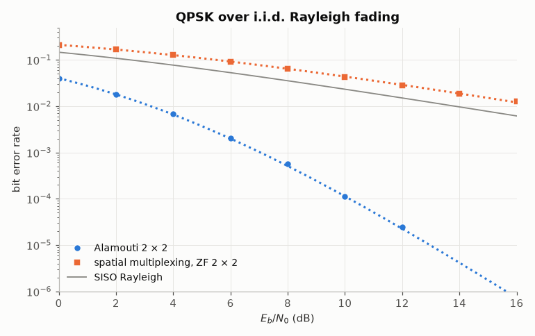
Diversity. Alamouti’s code over 2 × 2 Rayleigh fading (Alamouti 1998) collects the diversity of the four antenna pairs: its BER is that of maximal-ratio combining of four branches, 3 dB below in SNR since the power is split between the antennas. Spatial multiplexing with zero forcing doubles the rate but keeps \(n_r - n_t + 1 = 1\) branch (Winters, Salz & Gitlin 1994). The chain is that of specs/mimo_diversity.yaml; the dotted lines are the closed forms (Proakis & Salehi, eq. 13.4-15).

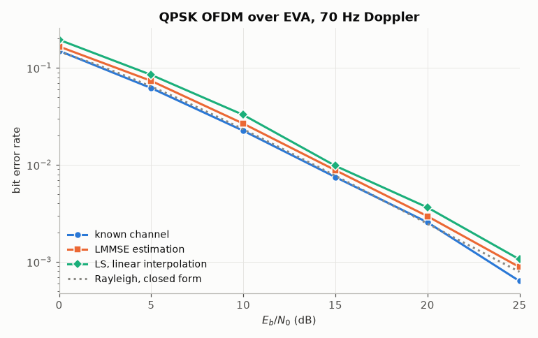
OFDM. Over the EVA channel of 3GPP TS 36.101 with a Doppler of 70 Hz, every subcarrier of an OFDM link is a flat Rayleigh channel: with the channel known, the BER is that of BPSK over Rayleigh fading. Estimating it from lattice pilots costs a fraction of a dB, less with LMMSE interpolation (Edfors et al. 1998) than with linear interpolation.

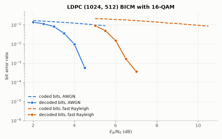
Coded modulation. A regular (3, 6) LDPC code of 1024 bits with 16-QAM and a random bit interleaver (BICM, Caire, Taricco & Biglieri 1998): over AWGN its waterfall is about 1.5 dB from the BICM limit; over fast Rayleigh fading the interleaved code collects the time diversity, where the BER of the coded bits only falls as \(1/\mathrm{SNR}\).

import matplotlib.pyplot as plt
import numpy as np

# the BICM chain is shared with the test that checks these curves
from _gallery_utils import SPECS, bicm_chain

import comnum
from comnum import blocks as B
from comnum.plot import BACKGROUND, BLUE, GREY, RUST


def rate(results, metric, **condition):
    """The values of a rate metric against E_b/N_0, NaN below 20 errors."""
    return results.series("ebn0_db", metric, min_count=20, **condition)[1]

Diversity of two transmit antennas over 2 × 2 Rayleigh fading.

eb = np.arange(0.0, 17.0, 2.0)
link = comnum.Chain.from_spec(SPECS / "mimo_diversity.yaml")
res = link.run(
    grid={"scheme": ["alamouti", "spatial"], "ebn0_db": list(eb)},
    stop={"min_errors": {"ber": 200}, "min_trials": 4, "max_trials": 400},
)
fig, ax = plt.subplots()
fine = np.linspace(0, 16, 81)
for scheme, branches, marker, label in [
    ("alamouti", 4, "o", "Alamouti 2 × 2"),
    ("spatial", 1, "s", "spatial multiplexing, ZF 2 × 2"),
]:
    (line,) = ax.semilogy(
        eb, rate(res, "ber", scheme=scheme), marker=marker, markeredgecolor=BACKGROUND,
        linestyle="none", label=label,
    )  # fmt: skip
    ax.semilogy(
        fine,
        comnum.theory_ber_rayleigh_mrc(fine - comnum.lin2db(2), branches=branches),
        ":",
        color=line.get_color(),
    )
ax.semilogy(
    fine,
    comnum.theory_ber_rayleigh_mrc(fine, branches=1),
    color=GREY,
    linewidth=1.2,
    label="SISO Rayleigh",
)
ax.set(
    xlabel="$E_b/N_0$ (dB)", ylabel="bit error rate", ylim=(1e-6, 0.5), xlim=(0, 16),
    title="QPSK over i.i.d. Rayleigh fading",
)  # fmt: skip
ax.legend(loc="lower left")
fig.tight_layout()

OFDM over EVA: known channel, LMMSE and linear interpolation of the pilots.

eb = np.arange(0.0, 26.0, 5.0)
lattice = {"pattern": "lattice", "freq": 3, "time": 4}
ofdm = comnum.Chain(
    tx=B.Source(constellation="QPSK", n_symbols=2400),
    ofdm=B.OfdmTx(n_fft=256, n_subcarriers=200, n_cp=18, pilots=lattice),
    channel=B.Tdl(profile="EVA", doppler_hz=70),
    noise=B.AwgnEbn0(ebn0_db=comnum.var("ebn0_db")),
    rx=B.OfdmRx(estimation=comnum.var("estimation"), detector="zf"),
)
res = ofdm.run(
    grid={"estimation": ["perfect", "lmmse", "ls"], "ebn0_db": list(eb)},
    metrics={"report": ["ber"], "scale": "none"},
    stop={"min_trials": 300, "max_trials": 300},
)
fig, ax = plt.subplots()
for est, marker, label in [
    ("perfect", "o", "known channel"),
    ("lmmse", "s", "LMMSE estimation"),
    ("ls", "D", "LS, linear interpolation"),
]:
    ax.semilogy(
        eb, rate(res, "ber", estimation=est), marker=marker, markeredgecolor=BACKGROUND,
        label=label,
    )  # fmt: skip
ax.semilogy(fine := np.linspace(0, 25, 101), comnum.theory_ber_rayleigh_mrc(fine, branches=1), ":",
            color=GREY, label="Rayleigh, closed form")  # fmt: skip
ax.set(
    xlabel="$E_b/N_0$ (dB)", ylabel="bit error rate", xlim=(0, 25),
    title="QPSK OFDM over EVA, 70 Hz Doppler",
)  # fmt: skip
ax.legend(loc="lower left")
fig.tight_layout()

BICM: an LDPC code of 1024 bits with 16-QAM over AWGN and fast Rayleigh fading: FecEncode(code, blocks=4, interleave=True), Map("16-QAM"), with fading Rayleigh(coherence_samples=1), AwgnEbn0, with fading MimoRx, Demap and FecDecode (bicm_chain).

fig, ax = plt.subplots()
for fading, eb, color, name in [
    (False, np.arange(2.0, 5.6, 0.5), BLUE, "AWGN"),
    (True, np.arange(5.0, 10.6, 0.5), RUST, "fast Rayleigh"),
]:
    res = bicm_chain(fading).run(
        grid={"ebn0_db": list(eb)},
        metrics=["ber", "coded_ber"],
        stop={"min_errors": {"coded_ber": 200}, "min_trials": 4, "max_trials": 400},
    )
    ax.semilogy(eb, rate(res, "ber"), "--", color=color, label=f"coded bits, {name}")
    ax.semilogy(
        eb, rate(res, "coded_ber"), "o-", color=color, markeredgecolor=BACKGROUND,
        label=f"decoded bits, {name}",
    )  # fmt: skip
ax.set(
    xlabel="$E_b/N_0$ (dB)", ylabel="bit error rate", ylim=(1e-6, 0.5),
    title="LDPC (1024, 512) BICM with 16-QAM",
)  # fmt: skip
ax.legend(loc="lower left")
fig.tight_layout()