Optical wireless: an LED-lit room and a turbulent free-space link

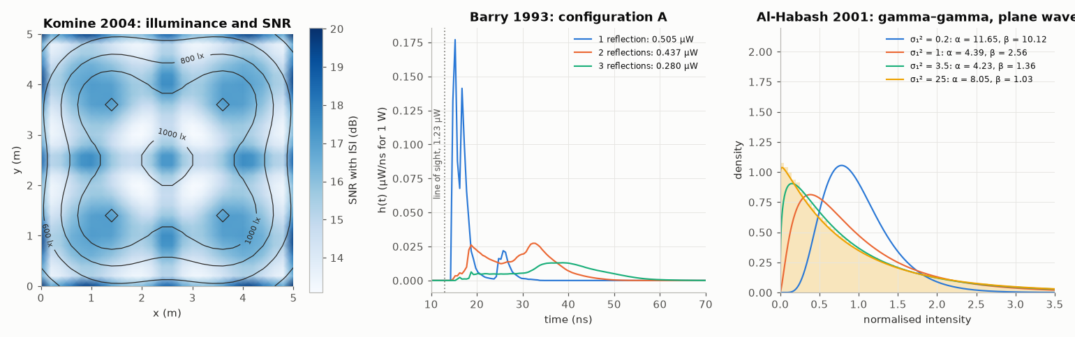
Light as the medium outside the fibre, in three panels to open next to the figures of the papers they reproduce.

1. Illuminance and SNR of a visible-light room. T. Komine and M. Nakagawa, “Fundamental analysis for visible-light communication system using LED lights,” IEEE Trans. Consum. Electron. 50(1), 2004, Figs. 3 and 9: four lights of 60 × 60 LEDs (20 mW, semi-angle 70°) in a 5 × 5 × 3 m room, a desk 0.85 m high, a photodiode of 1 cm² with a field of view of 60° (comnum.OwcRoom). The contours are the illuminance (313.5 to 1211.5 lx); the colour is the SNR of 100 Mb/s on–off keying with the reflections of the walls (\(\rho = 0.7\)) and the PIN-FET receiver of their Table II (comnum.PinFetReceiver): the interference between symbols, not the noise, sets it.

2. Multipath of an infrared link. J. R. Barry, J. M. Kahn, W. J. Krause, E. A. Lee and D. G. Messerschmitt, IEEE J. Sel. Areas Commun. 11(3), 1993, Fig. 3 (configuration A): the impulse response of a source on the ceiling, by order of reflection, computed recursively on the elements of the walls (with partitions coarser than their Table I, for speed: the second and third orders come out 2 and 4 % above their 0.430 and 0.269 µW).

3. Turbulence. M. A. Al-Habash, L. C. Andrews and R. L. Phillips, Opt. Eng. 40(8), 2001: the gamma–gamma density of the intensity of a plane wave (comnum.GammaGamma.from_rytov) from weak (Rytov variance 0.2) to saturated turbulence, the last one that of their Fig. 3 (Rytov variance 25, \(\alpha = 8.05\), \(\beta = 1.03\)), against a histogram of draws.

validation/tests/optical_wireless/komine2004.rs, barry1993.rs and alhabash2001.rs check the same values with tolerances (docs/LITERATURE.md lists the gaps that remain).

import matplotlib.pyplot as plt
import numpy as np

import comnum
from comnum.plot import GREY, LABEL, MUTED

fig, axes = plt.subplots(1, 3, figsize=(14, 4.4), width_ratios=[1.15, 1, 1])

# 1. the room of Komine & Nakagawa
off = (np.arange(60) - 29.5) * 0.01
lights = [(1.25, 1.25), (3.75, 1.25), (1.25, 3.75), (3.75, 3.75)]
chips = np.array([(cx + a, cy + b, 2.5) for cx, cy in lights for a in off for b in off])
down, up = [0.0, 0.0, -1.0], [0.0, 0.0, 1.0]
mode = comnum.lambertian_mode(np.radians(70))
walls = {"north": 0.7, "south": 0.7, "east": 0.7, "west": 0.7}
lit = comnum.OwcRoom([5.0, 5.0, 3.0], walls).illuminate(
    chips, down, mode, 20e-3, bin_s=0.01e-9, partitions=[[50, 50, 30]]
)
rx = comnum.PinFetReceiver.komine2004()
xs = np.linspace(0, 5, 26)
lux = np.zeros((xs.size, xs.size))
snr = np.zeros_like(lux)
for i, x in enumerate(xs):
    for j, y in enumerate(xs):
        point = [x, y, 0.85]
        lux[j, i] = comnum.owc_illuminance(chips, down, mode, 0.73, point, up)
        h = lit.impulse_responses(point, up, 1e-4, np.radians(60), concentrator_index=1.5)
        both = h[0] + h[1]
        s, isi = both.bit_split(10e-9, h[0].first_arrival_s())
        snr[j, i] = rx.ook_snr_db(s, isi, 1e-4, 100e6)
ax = axes[0]
image = ax.pcolormesh(xs, xs, snr, cmap="Blues", shading="gouraud")
fig.colorbar(image, ax=ax, label="SNR with ISI (dB)")
contours = ax.contour(xs, xs, lux, levels=[400, 600, 800, 1000, 1200], colors=LABEL, linewidths=0.8)
ax.clabel(contours, fmt="%d lx", fontsize=7)
ax.set(xlabel="x (m)", ylabel="y (m)", title="Komine 2004: illuminance and SNR", aspect=1)
ax.grid(False)

# 2. configuration A of Barry et al., by order of reflection
rho = {"north": 0.8, "south": 0.8, "east": 0.8, "west": 0.8, "ceiling": 0.8, "floor": 0.3}
lit = comnum.OwcRoom([5.0, 5.0, 3.0], rho).illuminate(
    [2.5, 2.5, 3.0],
    down,
    1.0,
    1.0,
    bin_s=0.5e-9,
    partitions=[[50, 50, 30], [25, 25, 15], [15, 15, 9]],
)
h = lit.impulse_responses([0.5, 1.0, 0.0], up, 1e-4, np.radians(85))
ax = axes[1]
for k, r in enumerate(h[1:], start=1):
    t = (np.arange(r.power_w.size) + 0.5) * r.bin_s * 1e9
    ax.plot(
        t,
        r.power_w / r.bin_s * 1e-3,
        linewidth=1.4,
        label=f"{k} reflection{'s' if k > 1 else ''}: {r.total_w() * 1e6:.3f} µW",
    )
ax.axvline(h[0].first_arrival_s() * 1e9, color=GREY, linestyle=":", linewidth=1.2)
ax.text(
    h[0].first_arrival_s() * 1e9 - 0.6,
    0.5 * ax.get_ylim()[1],
    f"line of sight, {h[0].total_w() * 1e6:.2f} µW",
    fontsize=8,
    color=MUTED,
    rotation=90,
    ha="right",
    va="center",
)
ax.set(
    xlim=(10, 70),
    xlabel="time (ns)",
    ylabel="h(t) (µW/ns for 1 W)",
    title="Barry 1993: configuration A",
)
ax.legend(loc="upper right", fontsize=8)

# 3. gamma-gamma densities of Al-Habash et al.
ax = axes[2]
i = np.linspace(1e-3, 3.5, 600)
for rytov in [0.2, 1.0, 3.5, 25.0]:
    g = comnum.GammaGamma.from_rytov(rytov)
    (line,) = ax.plot(
        i, g.pdf(i), linewidth=1.4, label=f"σ₁² = {rytov:g}: α = {g.alpha:.2f}, β = {g.beta:.2f}"
    )
g = comnum.GammaGamma.from_rytov(25.0)
draws = g.draw(200_000, comnum.Rng(2001))
ax.hist(
    draws,
    bins=np.linspace(0, 3.5, 71),
    density=True,
    color=line.get_color(),
    alpha=0.25,
    linewidth=0,
)
ax.set(
    xlim=(0, 3.5),
    ylim=(0, 2.2),
    xlabel="normalised intensity",
    ylabel="density",
    title="Al-Habash 2001: gamma–gamma, plane wave",
)
ax.legend(loc="upper right", fontsize=8)
fig.tight_layout()
plt.show()