
Note
Go to the end to download the full example code.
DAC and ADC: quantisation, clipping and jitter#
A converter of \(N\) bits and full scale \(A\) rounds every in-phase and
quadrature sample to one of \(2^N\) levels spaced by \(\Delta = 2A/2^N\), and
clips beyond \(\pm A\). comnum.adc and comnum.dac model it, with an analogue
bandwidth, the noise of an effective number of bits (ENOB), the sampling-clock jitter
(ADC) and the zero-order hold (DAC); the adc and dac blocks put them in a link.
Every curve below is checked against its closed form by
validation/tests/hardware/converters.rs:
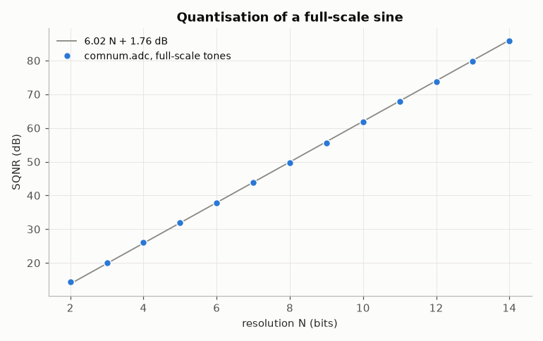
the granular noise \(\Delta^2/12\) and the SQNR of a full-scale sine, \(6.02 N + 1.76\) dB (Bennett, Bell Syst. Tech. J. 27(3), 1948);
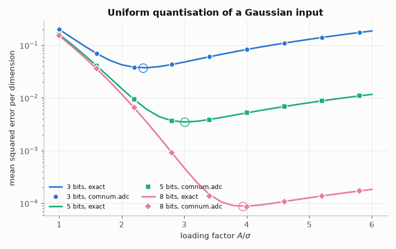
the exact error of a Gaussian input, granular plus overload, and the loading factor \(A/\sigma\) that minimises it (the optimal uniform quantiser of Max, IRE Trans. Inf. Theory 6(1), 1960);
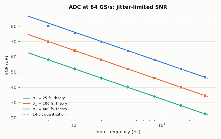
the SNR limited by a clock jitter \(\sigma_j\), \(-20 \log_{10}(2\pi f \sigma_j)\) (Walden, IEEE J. Sel. Areas Commun. 17(4), 1999);
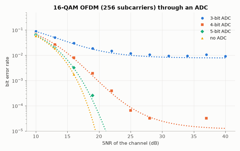
the BER of an OFDM link through an ADC: the channel noise plus the quantisation noise.
import matplotlib.pyplot as plt
import numpy as np

import comnum
from comnum.plot import BACKGROUND, GREY

rng = comnum.Rng(1)
The SQNR of a sine#
A complex tone of amplitude close to full scale, at a frequency incommensurate with the sampling, averaged over a few tones (the error of one deterministic sine strays by a few tenths of a dB from the formula).
bits_range = np.arange(2, 15)
measured = []
for bits in bits_range:
    noise = 0.0
    for _ in range(8):
        f = 0.01 + 0.48 * rng.uniform(1)[0]
        a = 0.95 + 0.05 * rng.uniform(1)[0]
        n = np.arange(1 << 14)
        x = a * np.exp(2j * np.pi * f * n)
        y = comnum.adc(x, int(bits), full_scale=1.0)
        c = np.mean(y * np.exp(-2j * np.pi * f * n))
        noise += np.mean(np.abs(y - c * np.exp(2j * np.pi * f * n)) ** 2) / a**2
    measured.append(comnum.lin2db(8 / noise))

fig, ax = plt.subplots()
ax.plot(bits_range, [comnum.theory_sqnr_sine_db(int(b)) for b in bits_range], color=GREY,
        linewidth=1.2, label="6.02 N + 1.76 dB")  # fmt: skip
ax.plot(bits_range, measured, "o", markeredgecolor=BACKGROUND, label="comnum.adc, full-scale tones")
ax.set(xlabel="resolution N (bits)", ylabel="SQNR (dB)", title="Quantisation of a full-scale sine")
ax.legend()
fig.tight_layout()
A Gaussian input: granular noise against clipping#
An OFDM signal is Gaussian per dimension. A small full scale clips often; a large one makes the steps coarse. The exact error (lines) is the sum of the two; the points are simulated; the circles mark the optimal loading, which grows slowly with the resolution.
x = rng.complex_noise(200_000, 2.0)  # unit variance per dimension
loadings = np.linspace(1.0, 6.0, 26)
fig, ax = plt.subplots()
for bits, marker in zip([3, 5, 8], ["o", "s", "D"], strict=True):
    theory = [comnum.theory_quantization_mse(bits, lam) for lam in loadings]
    (line,) = ax.semilogy(loadings, theory, label=f"{bits} bits, exact")
    sim = [
        np.mean(np.abs(comnum.adc(x, bits, full_scale=lam) - x) ** 2) / 2 for lam in loadings[::3]
    ]
    ax.semilogy(loadings[::3], sim, marker, color=line.get_color(), markeredgecolor=BACKGROUND,
                label=f"{bits} bits, comnum.adc")  # fmt: skip
    best = comnum.optimal_loading(bits)
    ax.semilogy([best], [comnum.theory_quantization_mse(bits, best)], "o", markersize=11,
                markerfacecolor="none", markeredgecolor=line.get_color())  # fmt: skip
ax.set(
    xlabel=r"loading factor $A/\sigma$",
    ylabel="mean squared error per dimension",
    title="Uniform quantisation of a Gaussian input",
)
ax.legend(ncols=2, fontsize=8)
fig.tight_layout()

print("bits   optimal loading   minimum error")
for bits in range(1, 9):
    lam = comnum.optimal_loading(bits)
    print(f"{bits:4d}   {lam:15.3f}   {comnum.theory_quantization_mse(bits, lam):13.3e}")
bits   optimal loading   minimum error
   1             1.596       3.634e-01
   2             1.991       1.188e-01
   3             2.344       3.744e-02
   4             2.682       1.154e-02
   5             3.010       3.495e-03
   6             3.330       1.040e-03
   7             3.640       3.043e-04
   8             3.938       8.769e-05
Clock jitter#
Sampling at \(t_n + \delta_n\) adds \(\delta_n x'(t_n)\): the noise grows with the frequency of the input. A 14-bit converter at 64 GS/s, so that the jitter dominates.
fs, n = 64e9, 1 << 14
freqs = np.array([0.5, 1, 2, 4, 8, 16, 30]) * 1e9
fig, ax = plt.subplots()
for jitter, marker in zip([25e-15, 100e-15, 400e-15], ["o", "s", "D"], strict=True):
    f_fine = np.geomspace(3e8, 3.2e10, 50)
    (line,) = ax.semilogx(f_fine, [comnum.theory_jitter_snr_db(f, jitter) for f in f_fine],
                          label=f"σ_j = {jitter * 1e15:.0f} fs, theory")  # fmt: skip
    snr = []
    for f in freqs:
        cycles = round(f / fs * n)  # a whole number of periods
        tone = np.exp(2j * np.pi * cycles / n * np.arange(n))
        y = comnum.adc(tone, 14, fs=fs, full_scale=1.05, jitter_s=jitter, rng=rng)
        c = np.mean(y * np.conj(tone))
        snr.append(comnum.lin2db(abs(c) ** 2 / np.mean(np.abs(y - c * tone) ** 2)))
    ax.semilogx(freqs, snr, marker, color=line.get_color(), markeredgecolor=BACKGROUND)
ax.axhline(comnum.theory_sqnr_sine_db(14), color=GREY, linestyle=":", linewidth=1.2,
           label="14-bit quantisation")  # fmt: skip
ax.set(xlabel="input frequency (Hz)", ylabel="SNR (dB)", title="ADC at 64 GS/s: jitter-limited SNR")
ax.legend(fontsize=8)
fig.tight_layout()
An OFDM link through an ADC#
16-QAM on 256 subcarriers over AWGN, converted at the optimal loading: the quantisation noise adds to the noise of the channel and the BER floors at the SNR of the converter (dotted lines: the closed form of 16-QAM at the total SNR; the clipping part of the noise is counted as additive).
c16 = comnum.Constellation("qam", 16).normalized()
snrs = np.arange(10.0, 41.0, 3.0)
fig, ax = plt.subplots()
for bits, marker in zip([3, 4, 5, None], ["o", "s", "D", "^"], strict=True):
    ber = []
    for snr in snrs:
        s2 = 1 / comnum.db2lin(snr)
        errors = total = 0
        for _ in range(30):
            b = rng.integers(2, 256 * 4).astype(np.uint8)
            x = np.fft.ifft(c16.map_bits(b)) * np.sqrt(256)
            y = x + rng.complex_noise(256, s2)
            if bits is not None:
                y = comnum.adc(y, bits)
            d = c16.demap_bits(np.fft.fft(y) / np.sqrt(256))
            errors += int(np.sum(d != b))
            total += b.size
        ber.append(errors / total)
    ber = np.array(ber)
    label = f"{bits}-bit ADC" if bits else "no ADC"
    keep = ber > 0
    (line,) = ax.semilogy(snrs[keep], ber[keep], marker, markeredgecolor=BACKGROUND, label=label)
    fine = np.linspace(10, 40, 61)
    if bits is None:
        total_noise = 1 / comnum.db2lin(fine)
    else:
        # the error per dimension of a unit-variance signal at the optimal loading, for
        # the signal and noise of variance (1 + σ²)/2 per dimension
        q = comnum.theory_quantization_mse(bits, comnum.optimal_loading(bits))
        total_noise = 1 / comnum.db2lin(fine) + 2 * q * (1 + 1 / comnum.db2lin(fine)) / 2
    ax.semilogy(
        fine,
        comnum.theory_ber(16, comnum.lin2db(1 / (4 * total_noise))),
        ":",
        color=line.get_color(),
    )
ax.set(
    ylim=(1e-5, 0.5),
    xlabel="SNR of the channel (dB)",
    ylabel="bit error rate",
    title="16-QAM OFDM (256 subcarriers) through an ADC",
)
ax.legend()
fig.tight_layout()
The zero-order hold of a DAC#
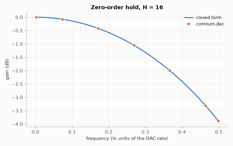
Holding every sample for \(H\) output samples filters the signal by \(\sin(\pi f/f_s)/(H \sin(\pi f/(H f_s)))\), close to \(\mathrm{sinc}(f/f_s)\): 3.9 dB of droop at the Nyquist frequency, which a transmitter pre-equalises.
n, hold = 1 << 12, 16
fr = np.linspace(0.0, 0.5, 200)
measured_f, measured_g = [], []
for cycles in [10, 300, 700, 1100, 1500, 1900, 2040]:
    f = cycles / n
    tone = np.exp(2j * np.pi * f * np.arange(n))
    y = comnum.dac(tone, 16, full_scale=1.05, hold=hold)
    c = np.mean(y * np.exp(-2j * np.pi * f / hold * np.arange(y.size)))
    measured_f.append(f)
    measured_g.append(20 * np.log10(abs(c)))
fig, ax = plt.subplots()
ax.plot(
    fr, [20 * np.log10(comnum.zero_order_hold_gain(f, 1.0, hold)) for f in fr], label="closed form"
)
ax.plot(measured_f, measured_g, "o", markeredgecolor=BACKGROUND, label="comnum.dac")
ax.set(
    xlabel="frequency (in units of the DAC rate)",
    ylabel="gain (dB)",
    title=f"Zero-order hold, H = {hold}",
)
ax.legend()
fig.tight_layout()
Total running time of the script: (0 minutes 0.902 seconds)