Ergodic capacity of MIMO channels

The capacity of a channel realisation with equal power on the \(n_t\) antennas is \(\log_2\det(I + \frac{\rho}{n_t} H H^H)\); its mean over Rayleigh fading grows like \(\min(n_t, n_r) \log_2 \rho\) at high SNR — one bit per 3 dB and per spatial stream (Foschini & Gans 1998, Telatar 1999). Water-filling on the eigenmodes, which needs the channel at the transmitter, helps at low SNR, where only the strongest modes deserve power. Antenna correlation (exponential, \(\rho = 0.9\)) removes part of the multiplexing gain.

import matplotlib.pyplot as plt
import numpy as np

import comnum

snr = np.arange(-10.0, 31.0, 2.5)
N = 4000
rng = comnum.Rng(17)
fig, ax = plt.subplots()
for n in [1, 2, 4]:
    h = comnum.mimo_channels(N, n, n, rng)
    (line,) = ax.plot(snr, [comnum.mimo_capacity(h, s).mean() for s in snr], label=f"{n} × {n}")
    if n == 4:
        ax.plot(
            snr,
            [comnum.mimo_capacity(h, s, water_filling=True).mean() for s in snr],
            color=line.get_color(),
            linestyle="--",
            linewidth=1.4,
            label="4 × 4, water-filling",
        )
        hc = comnum.mimo_channels(N, 4, 4, rng, rx_correlation=0.9, tx_correlation=0.9)
        ax.plot(
            snr,
            [comnum.mimo_capacity(hc, s).mean() for s in snr],
            color=line.get_color(),
            linestyle=":",
            linewidth=1.4,
            label=r"4 × 4, correlated ($\rho$ = 0.9)",
        )
ax.set(
    xlabel=r"SNR $\rho$ (dB)",
    ylabel="ergodic capacity (bit/s/Hz)",
    xlim=(-10, 30),
    ylim=(0, None),
    title="i.i.d. Rayleigh fading",
)
ax.legend()
fig.tight_layout()

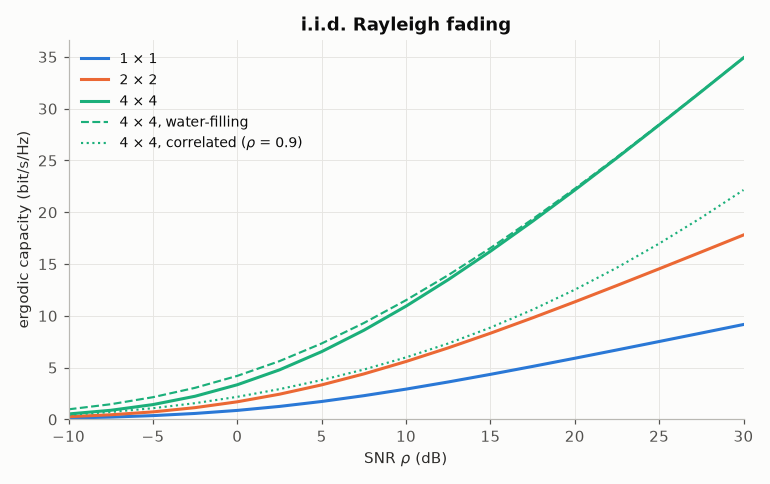
At 20 dB, the capacity of 4 × 4 is close to four times that of a single antenna.

h1, h4 = comnum.mimo_channels(N, 1, 1, rng), comnum.mimo_channels(N, 4, 4, rng)
c1, c4 = comnum.mimo_capacity(h1, 20.0).mean(), comnum.mimo_capacity(h4, 20.0).mean()
print(f"1 × 1: {c1:.2f} bit/s/Hz, 4 × 4: {c4:.2f} bit/s/Hz, ratio {c4 / c1:.2f}")

1 × 1: 5.86 bit/s/Hz, 4 × 4: 22.19 bit/s/Hz, ratio 3.78