Mach–Zehnder and IQ modulators#

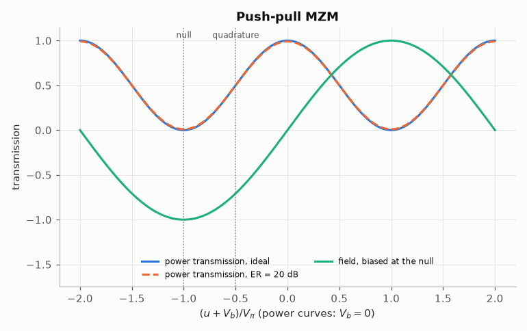
A Mach–Zehnder modulator (MZM) splits the optical field into two arms, shifts their phases with the driving voltage and recombines them. Driven in push-pull, the two arms move in opposite directions and the output field is real (no chirp):

\[E_{out} = E_{in} \left[c_I \cos\theta + j\, c_Q \sin\theta\right], \qquad \theta = \frac{\pi (u + V_b)}{2 V_\pi},\]

with $V_\pi$ the half-wave voltage, $V_b$ the bias and $c_I = \sqrt{r/(r+1)}$, $c_Q = 1/\sqrt{r+1}$ the arm coefficients of an extinction ratio $r$ ($c_I = 1, c_Q = 0$ for an ideal modulator). Two bias points matter:

the quadrature point $V_b = -V_\pi/2$, where the power responds linearly to small drives (intensity modulation);
the null $V_b = -V_\pi$, where the field is $\sin(\pi u / 2V_\pi)$, odd in the drive: the bias of coherent modulation (BPSK, the two arms of an IQ modulator).

comnum.mzm, comnum.iqm and comnum.phase_modulator follow the device models of OptiCommPy (tests/oracle/test_oracle.py compares them on the same inputs); tests/test_performance.py checks every closed form of this page.

import matplotlib.pyplot as plt
import numpy as np

import comnum
from comnum.plot import BACKGROUND, GREY, MUTED

VPI = 2.0


def bessel_j(k, x):
    """J_k(x) = (1/π) ∫_0^π cos(kτ - x sin τ) dτ (the trapezoidal rule is exact to
    rounding for this periodic integrand)."""
    tau = np.linspace(0.0, np.pi, 4001)
    return np.trapezoid(np.cos(k * tau - x * np.sin(tau)), tau) / np.pi

Transfer functions and bias points#

The power transmission $\cos^2\theta$ and, biased at the null, the field $\sin(\pi u/2V_\pi)$ against the drive. A finite extinction ratio keeps a floor of power $1/(r+1)$ at the null.

u = np.linspace(-2 * VPI, 2 * VPI, 801)
fig, ax = plt.subplots()
for er_db, style in [(np.inf, "-"), (20.0, "--")]:
    p = np.abs(comnum.mzm(np.ones(u.size), u, vpi=VPI, vb=0.0, er_db=er_db)) ** 2
    label = "ideal" if np.isinf(er_db) else f"ER = {er_db:.0f} dB"
    ax.plot(u / VPI, p, style, label=f"power transmission, {label}")
field = comnum.mzm(np.ones(u.size), u, vpi=VPI, vb=-VPI, er_db=np.inf).real
ax.plot(u / VPI, field, label="field, biased at the null")
for x, name in [(-0.5, "quadrature"), (-1.0, "null")]:
    ax.axvline(x, color=GREY, linestyle=":", linewidth=1.0)
    ax.annotate(name, (x, 1.03), ha="center", fontsize=8, color=MUTED)
ax.set(xlabel=r"$(u + V_b)/V_\pi$ (power curves: $V_b = 0$)", ylabel="transmission", ylim=(-1.75, 1.15),
       title="Push-pull MZM")  # fmt: skip
ax.legend(fontsize=8, loc="lower center", ncols=2)
fig.tight_layout()

Extinction ratio#

Sweeping the bias, the ratio of the largest to the smallest output power is the extinction ratio $r$ of the arm coefficients.

biases = np.linspace(-2 * VPI, 0.0, 2001)
fig, ax = plt.subplots()
print("configured ER (dB)   measured ER (dB)")
for er_db in (15.0, 25.0, 35.0):
    p = np.array(
        [
            abs(comnum.mzm(np.ones(1), np.zeros(1), vpi=VPI, vb=b, er_db=er_db)[0]) ** 2
            for b in biases
        ]
    )
    ax.plot(biases / VPI, comnum.lin2db(p), label=f"ER = {er_db:.0f} dB")
    print(f"{er_db:20.1f}   {comnum.lin2db(p.max() / p.min()):16.6f}")
ax.set(
    xlabel=r"bias $V_b/V_\pi$",
    ylabel="output power (dB)",
    ylim=(-40, 2),
    title="Power against the bias",
)
ax.legend()
fig.tight_layout()

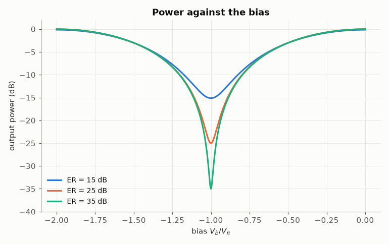
configured ER (dB)   measured ER (dB)
                15.0          15.000000
                25.0          25.000000
                35.0          35.000000

Intensity modulation: harmonics of a sine drive#

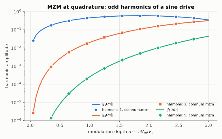
Biased at the quadrature point and driven by $V_m \sin x$, the power is $\frac{1}{2}(1 + \sin(m \sin x))$ with the modulation depth $m = \pi V_m/V_\pi$. The Jacobi–Anger expansion $\sin(m \sin x) = 2 \sum_{k\ \mathrm{odd}} J_k(m) \sin kx$ (Abramowitz & Stegun, Sec. 9.1) gives the amplitude $J_k(m)$ of every odd harmonic and none of the even ones: the third harmonic grows as $m^3$, the distortion that limits analogue links.

n, cycles = 4096, 8
x = 2 * np.pi * cycles * np.arange(n) / n
depths = np.linspace(0.05, 3.0, 60)
fig, ax = plt.subplots()
for k, marker in zip([1, 3, 5], ["o", "s", "D"], strict=True):
    (line,) = ax.semilogy(depths, [abs(bessel_j(k, m)) for m in depths], label=f"$|J_{k}(m)|$")
    measured = []
    for m in depths[::6]:
        p = (
            np.abs(
                comnum.mzm(
                    np.ones(n), m * VPI / np.pi * np.sin(x), vpi=VPI, vb=-VPI / 2, er_db=np.inf
                )
            )
            ** 2
        )
        measured.append(abs(np.fft.rfft(p)[k * cycles]) * 2 / n)
    ax.semilogy(depths[::6], measured, marker, color=line.get_color(), markeredgecolor=BACKGROUND,
                label=f"harmonic {k}, comnum.mzm")  # fmt: skip
ax.set(xlabel=r"modulation depth $m = \pi V_m / V_\pi$", ylabel="harmonic amplitude", ylim=(1e-6, 1),
       title="MZM at quadrature: odd harmonics of a sine drive")  # fmt: skip
ax.legend(ncols=2, fontsize=8)
fig.tight_layout()

MZM at quadrature: odd harmonics of a sine drive

IQ modulator: compression of 16-QAM and arcsine predistortion#

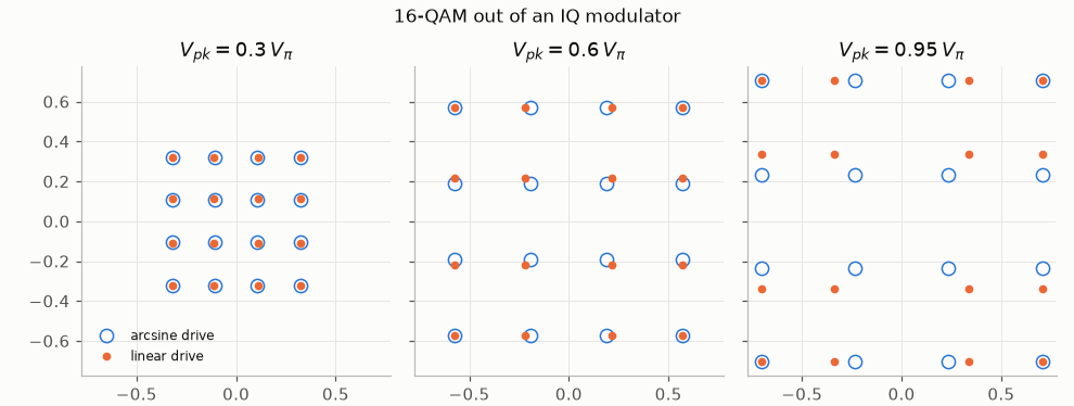
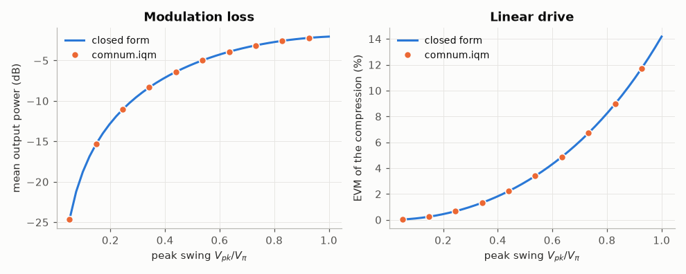
Two MZMs biased at the null, on the two halves of the field, recombined with a 90° phase: $E_{out} = \frac{E_{in}}{\sqrt{2}} [\sin(\pi u_I/2V_\pi) + j \sin(\pi u_Q/2V_\pi)]$. A linear drive of peak swing $V_{pk}$ compresses the outer levels of 16-QAM; a larger swing gives more power (less modulation loss) but more distortion. Driving with $u = \frac{2V_\pi}{\pi} \arcsin(s)$ makes the field proportional to the target $s$ exactly.

levels = np.array([-3.0, -1.0, 1.0, 3.0]) / 3
ui, uq = np.meshgrid(levels, levels)
s = (ui + 1j * uq).ravel()
ideal = dict(vpi=VPI, vb_i=-VPI, vb_q=-VPI, vphi=VPI / 2, er_i_db=np.inf, er_q_db=np.inf)

fig, axes = plt.subplots(1, 3, figsize=(9.0, 3.4), sharex=True, sharey=True)
for ax, swing in zip(axes, [0.3, 0.6, 0.95], strict=True):
    lin = comnum.iqm(np.ones(s.size), swing * VPI * s, **ideal)
    target = np.sin(np.pi * swing / 2) * s  # the same peak, without compression
    pre = comnum.iqm(
        np.ones(s.size),
        2 * VPI / np.pi * (np.arcsin(target.real) + 1j * np.arcsin(target.imag)),
        **ideal,
    )
    ax.plot(pre.real, pre.imag, "o", markerfacecolor="none", markersize=8, label="arcsine drive")
    ax.plot(lin.real, lin.imag, ".", markersize=8, label="linear drive")
    ax.set(title=f"$V_{{pk}} = {swing:g}\\, V_\\pi$", aspect="equal")
axes[0].legend(fontsize=8, loc="lower left")
fig.suptitle("16-QAM out of an IQ modulator", fontsize=11)
fig.tight_layout()

$16-QAM out of an IQ modulator, $V_{pk} = 0.3\, V_\pi$, $V_{pk} = 0.6\, V_\pi$, $V_{pk} = 0.95\, V_\pi$$

The trade-off, against the closed forms: the mean output power over the 16 points (in dB of the input) and the error of the linear drive with respect to an uncompressed constellation of the same mean power.

swings = np.linspace(0.05, 1.0, 40)
loss_theory, evm_theory, loss_sim, evm_sim = [], [], [], []
for swing in swings:
    a = np.sin(np.pi * swing * levels / 2)
    loss_theory.append(comnum.lin2db(np.mean(a**2)))  # (1/2) * 2 E[sin²] per point
    scaled = levels * np.sqrt(np.mean(a**2) / np.mean(levels**2))
    evm_theory.append(100 * np.sqrt(np.mean((a - scaled) ** 2) / np.mean(a**2)))
for swing in swings[::4]:
    e = comnum.iqm(np.ones(s.size), swing * VPI * s, **ideal)
    loss_sim.append(comnum.lin2db(np.mean(np.abs(e) ** 2)))
    ref = s * np.sqrt(np.mean(np.abs(e) ** 2) / np.mean(np.abs(s) ** 2))
    evm_sim.append(100 * np.sqrt(np.mean(np.abs(e - ref) ** 2) / np.mean(np.abs(e) ** 2)))

fig, (ax1, ax2) = plt.subplots(1, 2, figsize=(9.0, 3.6))
ax1.plot(swings, loss_theory, label="closed form")
ax1.plot(swings[::4], loss_sim, "o", markeredgecolor=BACKGROUND, label="comnum.iqm")
ax1.set(
    xlabel=r"peak swing $V_{pk}/V_\pi$", ylabel="mean output power (dB)", title="Modulation loss"
)
ax1.legend()
ax2.plot(swings, evm_theory, label="closed form")
ax2.plot(swings[::4], evm_sim, "o", markeredgecolor=BACKGROUND, label="comnum.iqm")
ax2.set(
    xlabel=r"peak swing $V_{pk}/V_\pi$", ylabel="EVM of the compression (%)", title="Linear drive"
)
ax2.legend()
fig.tight_layout()

Limits of the model#

The modulators are memoryless and chirp-free: the electrode bandwidth (a low-pass filter on the drive), the chirp of a single-drive MZM and the nonlinearity of the driver are not modelled. The first is a filter in a chain (comnum.blocks); the chirp of an unbalanced drive is the subject of Koyama & Iga, “Frequency chirping in external modulators” (J. Lightw. Technol., 1988), the reference a chirped model would be checked against.

Total running time of the script: (0 minutes 0.641 seconds)

Gallery generated by Sphinx-Gallery