Analysing a link: variants, probes and signals

The tools of the analysis after a campaign: comnum.compare() runs variants of a chain on the same grid, comnum.Results plots them with their confidence intervals and a closed form, probes measure inside the link during the campaign, and comnum.Chain.trace() with comnum.plot shows the signal after every block.

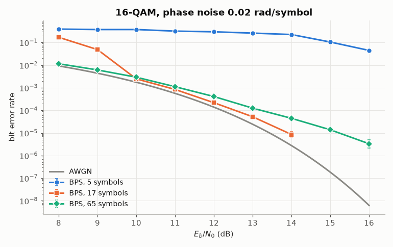
Variants. 16-QAM with Wiener phase noise (increments of 0.02 rad per symbol) and blind phase search (Pfau, Hoffmann & Noé 2009): a window of 5 symbols averages so little noise that the estimate slips by π/2 (cycle slips, after which every symbol is in error until the next slip); a long window averages the noise but lags the phase, and its errors fall slowly; the best window lies in between, within about 1 dB of the AWGN curve near a BER of 10⁻³.

Probes. LDPC-coded 16-QAM over fast Rayleigh fading: a probe after the MIMO detector measures the symbol error rate before decoding in the same campaign as the error rate after decoding.

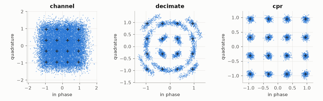
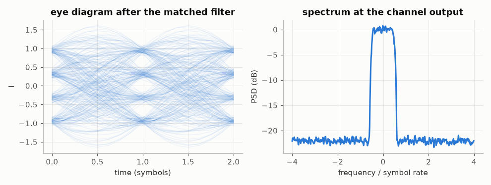
Signals. The constellation, the eye diagram and the spectrum after each block of a root-raised-cosine link with phase noise.

import matplotlib.pyplot as plt
import numpy as np

import comnum
from comnum import blocks as B
from comnum.plot import GREY

Variants: the window of blind phase search.

link = comnum.Chain(
    tx=B.Source(constellation="16-QAM", n_symbols=8192),
    pn=B.PhaseNoise(sigma_rad=0.02),
    ch=B.AwgnEbn0(ebn0_db=comnum.var("ebn0_db")),
    cpr=B.Bps(n=8, b=32),
    sync=B.FrameSync(length=256),
)
variants = {f"BPS, {2 * n + 1} symbols": link.replace(cpr=B.Bps(n=n, b=32)) for n in [2, 8, 32]}
res = comnum.compare(
    variants,
    grid={"ebn0_db": list(np.arange(8.0, 16.1, 1.0))},
    metrics={"report": ["ber"], "skip_start": 64, "skip_end": 64},
    stop={"min_errors": {"ber": 200}, "max_trials": 200},
)
ax = res.plot("ebn0_db", "ber", by="variant", min_count=20)
eb = np.linspace(8, 16, 81)
ax.semilogy(eb, comnum.theory_ber(16, eb, "qam"), color=GREY, label="AWGN")
ax.set(
    xlabel="$E_b/N_0$ (dB)", ylabel="bit error rate", title="16-QAM, phase noise 0.02 rad/symbol"
)
ax.legend(loc="lower left")
ax.figure.tight_layout()

Probes: the symbol errors before decoding and the bit errors after it, in one campaign.

code = {"type": "ldpc", "n": 1024, "k": 512, "seed": 1}
bicm = comnum.Chain(
    enc=B.FecEncode(code=code, blocks=4, interleave=True),
    map=B.Map(constellation="16-QAM"),
    fading=B.Rayleigh(coherence_samples=1),
    noise=B.AwgnEbn0(ebn0_db=comnum.var("ebn0_db")),
    rx=B.MimoRx(),
    demap=B.Demap(),
    dec=B.FecDecode(code=code, interleave=True),
).probe("rx", ["ser"], scale="none")
res = bicm.run(
    grid={"ebn0_db": list(np.arange(5.0, 9.1, 0.5))},
    metrics=["coded_ber"],
    stop={"min_errors": {"coded_ber": 100}, "min_trials": 4, "max_trials": 200},
)
print(res)
fig, ax = plt.subplots()
res.plot("ebn0_db", "rx.ser", ax=ax)
res.plot("ebn0_db", "coded_ber", ax=ax, min_count=20)
ax.legend(["symbol errors before decoding", "bit errors after decoding"], loc="lower left")
ax.set(
    xlabel="$E_b/N_0$ (dB)", ylabel="error rate", title="LDPC (1024, 512), 16-QAM, fast Rayleigh"
)
fig.tight_layout()

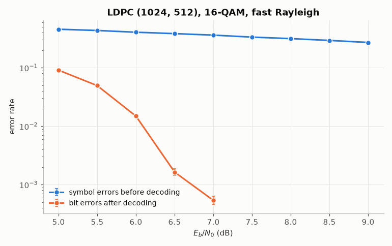
Results: 9 conditions, metrics ['coded_ber', 'rx.ser']
  (ebn0_db=5.0) 32 trials: coded_ber=0.091, rx.ser=0.4565
  (ebn0_db=5.5) 32 trials: coded_ber=0.04948, rx.ser=0.4348
  (ebn0_db=6.0) 32 trials: coded_ber=0.01489, rx.ser=0.4057
  (ebn0_db=6.5) 64 trials: coded_ber=0.00164, rx.ser=0.3843
  (ebn0_db=7.0) 128 trials: coded_ber=0.0005379, rx.ser=0.362
  (ebn0_db=7.5) 200 trials: coded_ber=0, rx.ser=0.3349
  (ebn0_db=8.0) 200 trials: coded_ber=0, rx.ser=0.3155
  (ebn0_db=8.5) 200 trials: coded_ber=0, rx.ser=0.2938
  (ebn0_db=9.0) 200 trials: coded_ber=0, rx.ser=0.2713

Signals: the frame after every block of one trial.

shaped = comnum.Chain(
    tx=B.Source(constellation="16-QAM", n_symbols=4096),
    shaping=B.PulseShape(sps=8, rolloff=0.2),
    channel=B.Awgn(snr_db=22.0),
    pn=B.PhaseNoise(sigma_rad=0.002),
    mf=B.MatchedFilter(rolloff=0.2),
    decimate=B.Decimate(),
    cpr=B.Bps(n=16, b=32),
)
frames = shaped.trace({}, comnum.Rng(3))
frames.plot("constellation", stages=["channel", "decimate", "cpr"], skip=256)

fig, (a, b) = plt.subplots(1, 2, figsize=(9, 3.4))
comnum.plot.eye(frames["mf"], ax=a, skip=1024)
a.set_title("eye diagram after the matched filter")
comnum.plot.psd(frames["channel"], ax=b, nfft=512)
b.set_title("spectrum at the channel output")
fig.tight_layout()

• 
•