Coverage of the confidence intervals of an error rate

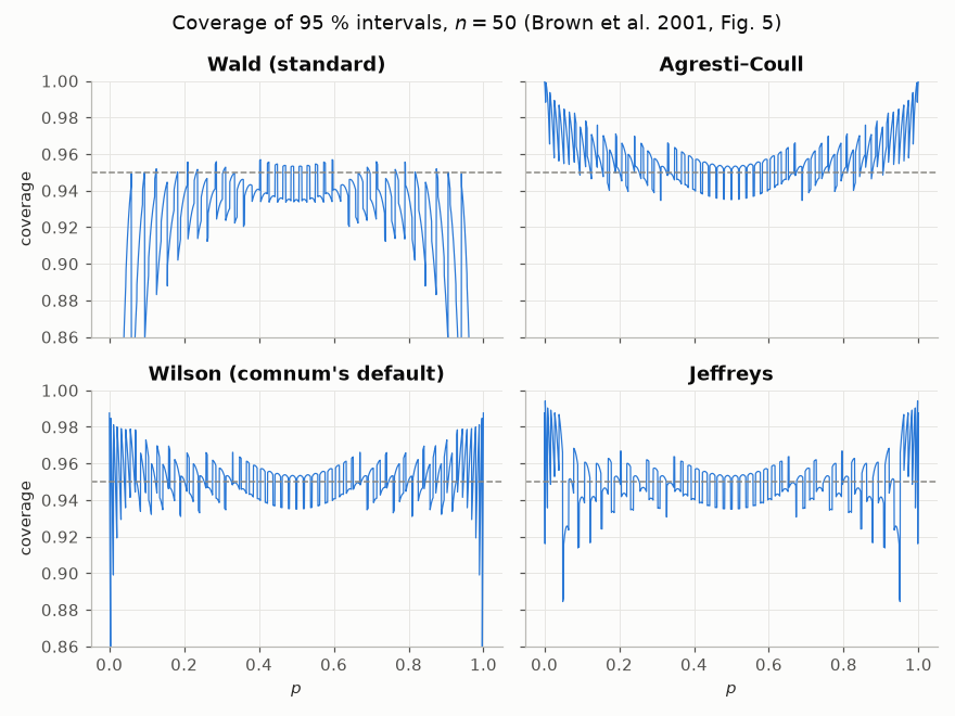
A Monte Carlo campaign estimates an error rate \(p\) from \(k\) errors among \(n\) trials and reports it with a confidence interval. The level of the interval, 95 % here, is only nominal: the probability that the interval actually contains \(p\), its coverage, depends on \(n\) and \(p\). For \(X \sim \mathrm{Bin}(n, p)\) it is the exact sum

\[C(p, n) = \sum_{k=0}^{n} \mathbf{1}\{L(k) \le p \le U(k)\} \binom{n}{k} p^{k} (1 - p)^{n - k},\]

computed by comnum.sim.interval_coverage() without simulation.

This example reproduces Fig. 5 of L. D. Brown, T. T. Cai and A. DasGupta, “Interval estimation for a binomial proportion,” Statistical Science 16(2), 101–133, 2001: the coverage of four intervals at \(n = 50\) on 2000 values of \(p\). The textbook (Wald) interval \(\hat p \pm z\sqrt{\hat p(1 - \hat p)/n}\) falls far below 0.95 near the ends and oscillates everywhere; the Wilson interval, the default of comnum’s runner, stays close to 0.95 except for narrow spikes near \(p = 0\) and 1; Agresti–Coull is slightly conservative; Jeffreys is close to Wilson. validation/tests/simulation/brown2001.rs checks the values of the paper behind this figure: the Wald coverages of its Tables 1 and 2 to the printed digits, the limits of its Sec. 3.2 and the 252 Jeffreys limits of its Table 5.

import math

import matplotlib.pyplot as plt
import numpy as np

from comnum import sim
from comnum.plot import GREY

n = 50
p = (np.arange(2000) + 0.5) / 2000
k = np.arange(n + 1)
# the binomial probabilities of k = 0..n for every p
log_choose = np.array([math.lgamma(n + 1) - math.lgamma(j + 1) - math.lgamma(n - j + 1) for j in k])
pmf = np.exp(log_choose + np.outer(np.log(p), k) + np.outer(np.log1p(-p), n - k))

methods = [
    ("wald", "Wald (standard)"),
    ("agresti_coull", "Agresti–Coull"),
    ("wilson", "Wilson (comnum's default)"),
    ("jeffreys", "Jeffreys"),
]
fig, axes = plt.subplots(2, 2, sharex=True, sharey=True, figsize=(8, 6))
for ax, (method, label) in zip(axes.flat, methods, strict=True):
    # the intervals of k = 0..n, computed once
    ends = np.array([sim.ErrorRate(int(j), n).interval(0.95, method=method) for j in k])
    covered = (ends[:, 0] <= p[:, None]) & (p[:, None] <= ends[:, 1])
    coverage = (pmf * covered).sum(axis=1)
    ax.plot(p, coverage, linewidth=0.8)
    ax.axhline(0.95, color=GREY, linestyle="--", linewidth=1.0)
    ax.set_title(label)
    ax.set_ylim(0.86, 1.0)
for ax in axes[1]:
    ax.set_xlabel("$p$")
for ax in axes[:, 0]:
    ax.set_ylabel("coverage")
fig.suptitle("Coverage of 95 % intervals, $n = 50$ (Brown et al. 2001, Fig. 5)")
fig.tight_layout()

The same numbers from the library: the coverage of the Wald interval at \(p = 1/2\) for \(n = 10\) is 0.891 (Table 1 of the paper), that of the Wilson interval 0.979.

print(
    round(sim.interval_coverage("wald", 10, 0.5), 3),
    round(sim.interval_coverage("wilson", 10, 0.5), 3),
)

0.891 0.979