WDM nonlinearity: the GN model and digital back-propagation

Dual-polarisation channels at 32 GBd propagated together by the Manakov equation (comnum.ManakovSsfm, the split step with the phase at the middle of the step), with EDFAs of noise figure 4.5 dB after every span of 80 km of standard fibre.

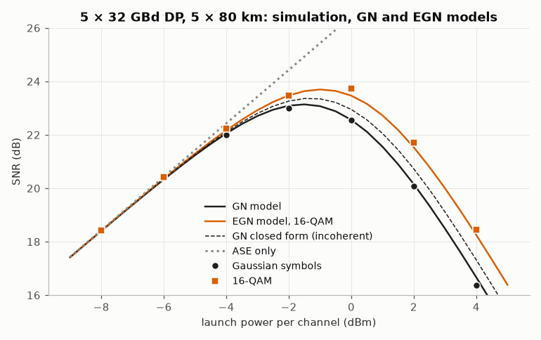
The GN model. Five channels on a 50 GHz grid over five spans: the SNR of the centre channel rises with the launch power while the ASE dominates, then falls by 2 dB per dB when the nonlinear interference, growing as \(P^3\), takes over. The GN model of Poggiolini (2012) treats the transmitted signal as Gaussian noise: Gaussian symbols follow it in both regimes (specs/wdm_gn.yaml checks it within 0.4 dB). 16-QAM generates less interference than Gaussian symbols: its SNR is about 1 dB above the GN model at the optimum and 1.5 dB above it beyond. The EGN model of Carena et al. (2014), the GN model corrected for the fourth and sixth moments of the constellation, follows it within 0.3 dB. Poggiolini’s closed form (incoherent accumulation of the spans) is close to the numerical integral.

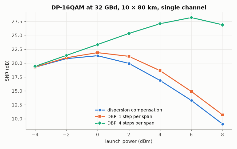
Back-propagation. A single channel over ten spans: dispersion compensation alone reaches its best SNR near 0 dBm; dual-polarisation digital back-propagation (comnum.ManakovSsfm.backpropagate(), Ip & Kahn 2008) with one step per span gains less than 1 dB at 32 GBd, while four steps per span remove most of the deterministic interference of the channel: the optimum moves about 6 dB higher and the SNR gains about 7 dB.

import matplotlib.pyplot as plt
import numpy as np
from _gallery_utils import SPECS

import comnum
from comnum import blocks as B
from comnum.plot import BACKGROUND, GREY, INK, RUST

The SNR of the centre channel against the launch power, simulated and GN model.

link = comnum.Chain.from_spec(SPECS / "wdm_gn.yaml")
powers = [-8.0, -6.0, -4.0, -2.0, 0.0, 2.0, 4.0]
res = link.run(grid={"format": ["gaussian", "16-QAM"], "power_dbm": powers}, stop={"max_trials": 4})
fiber = comnum.FiberParams(alpha_db_km=0.2, d_ps_nm_km=16, gamma_w_km=1.3, span_km=80, n_spans=5)
freqs = comnum.wdm_grid(5, 50e9)
fine = np.linspace(-9, 5, 29)
gn = [comnum.gn_model(fiber, freqs, p, 32e9, rolloff=0.1) for p in fine]
ase = np.array([g["ase_psd"] for g in gn]) * 32e9
closed = np.array([comnum.gn_closed_form(fiber, 5, 32e9, 50e9, p) for p in fine]) * 32e9
p_w = comnum.dbm2w(fine)

fig, ax = plt.subplots()
ax.plot(fine, [g["snr_db"] for g in gn], color=INK, linewidth=1.6, label="GN model")
egn = [
    comnum.gn_model(fiber, freqs, p, 32e9, rolloff=0.1, modulation="16-QAM")["snr_db"] for p in fine
]
ax.plot(fine, egn, color=RUST, linewidth=1.6, label="EGN model, 16-QAM")
ax.plot(fine, comnum.lin2db(p_w / (ase + closed)), "--", color=INK, linewidth=1.0,
        label="GN closed form (incoherent)")  # fmt: skip
ax.plot(fine, comnum.lin2db(p_w / ase), ":", color=GREY, label="ASE only")
for fmt, marker, color, label in [("gaussian", "o", INK, "Gaussian symbols"),
                                  ("16-QAM", "s", RUST, "16-QAM")]:  # fmt: skip
    _, snr = res.series("power_dbm", "snr_db", format=fmt)
    ax.plot(powers, snr, marker=marker, color=color, markeredgecolor=BACKGROUND, linestyle="none",
            label=label)  # fmt: skip
ax.set(
    xlabel="launch power per channel (dBm)", ylabel="SNR (dB)", ylim=(16, 26),
    title="5 × 32 GBd DP, 5 × 80 km: simulation, GN and EGN models",
)  # fmt: skip
ax.legend(loc="lower center")
fig.tight_layout()

Dispersion compensation against dual-polarisation back-propagation, one channel over ten spans.

single = comnum.Chain(
    tx=B.Source(constellation="16-QAM", n_symbols=4096, symbol_rate=32e9, pols=2),
    wdm=B.WdmTx(n_channels=1, sps=4, power_dbm=comnum.var("power_dbm"), rolloff=0.1),
    fiber=B.Manakov(),
    rx=B.WdmRx(sps=2),
    comp=B.Cdc(),
    mf=B.MatchedFilter(rolloff=0.1),
    dec=B.Decimate(),
    sync=B.FrameSync(start=1024, length=512, max_delay=16, symmetry=0),
)
long_haul = {"n_spans": 10, "span_km": 80, "d_ps_nm_km": 16, "gamma_w_km": 1.3}
powers = [-4.0, -2.0, 0.0, 2.0, 4.0, 6.0, 8.0]
fig, ax = plt.subplots()
for comp, marker, label in [
    (B.Cdc(), "o", "dispersion compensation"),
    (B.ManakovDbp(steps_per_span=1), "s", "DBP, 1 step per span"),
    (B.ManakovDbp(steps_per_span=4), "D", "DBP, 4 steps per span"),
]:
    res = single.replace(comp=comp).run(
        grid={"power_dbm": powers},
        metrics={"report": ["snr_db"], "skip_start": 256, "skip_end": 256},
        stop={"max_trials": 2},
        fiber=long_haul,
    )
    ax.plot(powers, res.series("power_dbm", "snr_db")[1], marker=marker,
            markeredgecolor=BACKGROUND, label=label)  # fmt: skip
ax.set(
    xlabel="launch power (dBm)", ylabel="SNR (dB)",
    title="DP-16QAM at 32 GBd, 10 × 80 km, single channel",
)  # fmt: skip
ax.legend(loc="lower center")
fig.tight_layout()