Recorded signals: SigMF in, blind receiver out

SigMF (the Signal Metadata Format, <sigmf/SigMF>) is the open format of the software-defined radio community: a JSON file name.sigmf-meta (the sample format, the sampling rate, the centre frequency of every capture, annotations) next to the raw samples name.sigmf-data, or both in a .sigmf archive. GNU Radio, inspectrum, SDRangel and most SDR tools read and write it.

comnum.read_sigmf() reads SigMF 1.x: every sample format ([c|r][f32|f64|i32|i16|i8|u32|u16|u8][_le|_be]), several channels, the header bytes of the captures, archives; comnum.write_sigmf() writes a recording with its centre frequency and annotations. tests/test_sigmf.py checks both directions against sigmf-python, the reference implementation. In a specification, the capture block plays the segments of a recording through a receiver chain, Monte Carlo style.

Below, a recording as an SDR would produce it, then a receiver that knows nothing of the signal: the symbol rate, the frequency offset, the modulation and the SNR all come from the samples.

import os
import tempfile

import matplotlib.pyplot as plt
import numpy as np

import comnum
from comnum.plot import BLUE, GREY

A recording

16-QAM at 270 kBd, root-raised-cosine roll-off 0.35, sampled at 1 MS/s (3.7 samples per symbol, not an integer), a carrier offset of 2.7 kHz, an SNR of 18 dB in the band of the symbol rate, 16-bit integers at -12 dBFS, the centre frequency (915 MHz) and an annotation of the occupied band.

RS, FS, CFO, FC = 270e3, 1e6, 2.7e3, 915e6
rng = comnum.Rng(29)
qam16 = comnum.Constellation("qam", 16).normalized()
_, a = comnum.symbols(qam16, 20_000, rng)
x8 = comnum.fir_filter(
    comnum.pulse_shape("rrc", 8, n_taps=8 * 32 + 1, rolloff=0.35), comnum.upsample(a, 8)
)
x = comnum.resample_fft(x8, round(x8.size * FS / (8 * RS)))
x = comnum.awgn(comnum.freq_shift(x, CFO, FS), 18.0, rng, fs=FS, bandwidth_hz=RS)
x = x / np.sqrt(np.mean(np.abs(x) ** 2)) * 0.25 * 32767

base = os.path.join(tempfile.mkdtemp(), "capture")
edges = {"freq_lower_edge": FC - 0.675 * RS, "freq_upper_edge": FC + 0.675 * RS}
comnum.write_sigmf(
    base,
    x,
    FS,
    datatype="ci16_le",
    fc_hz=FC,
    annotations=[{"sample_start": 0, "sample_count": x.size, "label": "16-QAM", **edges}],
    global_meta={"core:description": "16-QAM at 270 kBd", "core:hw": "comnum simulation"},
)
print(open(base + ".sigmf-meta", encoding="utf-8").read())

{
  "global": {
    "core:datatype": "ci16_le",
    "core:sample_rate": 1000000.0,
    "core:version": "1.2.0",
    "core:recorder": "comnum 0.3.1",
    "core:description": "16-QAM at 270 kBd",
    "core:hw": "comnum simulation"
  },
  "captures": [
    {
      "core:sample_start": 0,
      "core:frequency": 915000000.0
    }
  ],
  "annotations": [
    {
      "core:sample_start": 0,
      "core:sample_count": 74074,
      "core:label": "16-QAM",
      "core:freq_lower_edge": 914817750.0,
      "core:freq_upper_edge": 915182250.0
    }
  ]
}

Reading it back

autoscale=True divides the integers by their full scale, as sigmf-python does; the metadata come as a dictionary. The spectrum shows the annotated band, offset by the carrier error.

y, fs, meta = comnum.read_sigmf(base, autoscale=True)
fc = meta["captures"][0]["core:frequency"]
ann = meta["annotations"][0]
print(f"{y.size} samples at {fs / 1e6:g} MS/s, centre {fc / 1e6:g} MHz, label {ann['core:label']}")

n = 1024
seg = y[: y.size // n * n].reshape(-1, n) * np.hanning(n)
psd = np.fft.fftshift(np.mean(np.abs(np.fft.fft(seg, axis=1)) ** 2, axis=0))
f = (fc + np.fft.fftshift(np.fft.fftfreq(n, 1 / fs))) / 1e6
fig, ax = plt.subplots(figsize=(6.4, 3.2))
ax.plot(f, comnum.lin2db(psd / psd.max()), color=BLUE, linewidth=1)
ax.axvspan(
    ann["core:freq_lower_edge"] / 1e6,
    ann["core:freq_upper_edge"] / 1e6,
    color=GREY,
    alpha=0.15,
)
ax.set(xlabel="frequency (MHz)", ylabel="PSD (dB)", ylim=(-45, 3))
ax.grid(alpha=0.3)
fig.tight_layout()

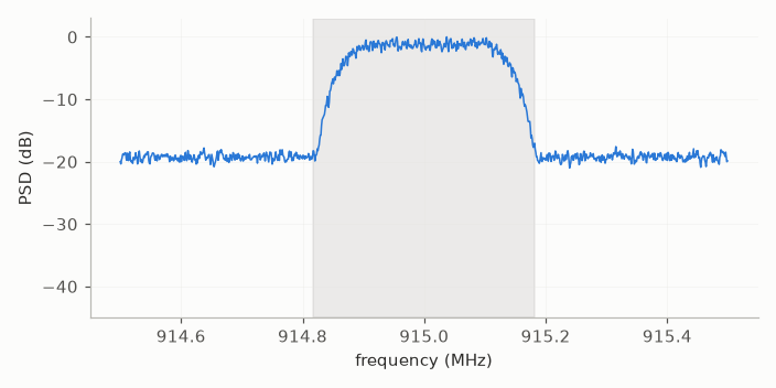
74074 samples at 1 MS/s, centre 915 MHz, label 16-QAM

A blind receiver

1. the symbol rate from the line of \(|x|^2\) (comnum.estimate_symbol_rate(), Gardner 1991);

2. resampling to two samples per symbol, the matched filter, Gardner’s clock recovery, and the strobe phase whose amplitudes are the most compact;

3. the carrier offset by the fourth power (comnum.fourth_power_foe()) and the phase by Viterbi–Viterbi, both blind for square QAM;

4. the modulation by the likelihood with the scale and the noise estimated (comnum.classify_modulation()), and the SNR by M2M4 (comnum.snr_m2m4_db()).

y = y / np.sqrt(np.mean(np.abs(y) ** 2))
rs = comnum.estimate_symbol_rate(y, fs, fs / 20, fs / 2)
z = comnum.resample_fft(y, round(y.size * 2 * rs / fs))
z = comnum.fir_filter(comnum.pulse_shape("rrc", 2, n_taps=2 * 32 + 1, rolloff=0.35), z)
z, _ = comnum.gardner_clock_recovery(z)


def kurtosis(s):
    return np.mean(np.abs(s) ** 4) / np.mean(np.abs(s) ** 2) ** 2


s = min((z[o::2] for o in (0, 1)), key=kurtosis)[200:-200]
s, cfo = comnum.fourth_power_foe(s, rs)
s = comnum.derotate(s, comnum.unwrap(comnum.viterbi_viterbi(s, n=32, m=4), period=np.pi / 2))
s = s / np.sqrt(np.mean(np.abs(s) ** 2))

names = ["BPSK", "QPSK", "8-PSK", "16-QAM", "64-QAM"]
cands = [
    comnum.Constellation(k, m).normalized()
    for k, m in [("psk", 2), ("qam", 4), ("psk", 8), ("qam", 16), ("qam", 64)]
]
decided = comnum.classify_modulation(s, cands)["index"]
snr = comnum.snr_m2m4_db(s, cands[decided])
print(f"symbol rate {rs / 1e3:.3f} kBd (true 270), offset {cfo / 1e3:.3f} kHz (true 2.7)")
print(
    f"modulation {names[decided]} (annotation {ann['core:label']}), SNR {snr:.1f} dB (18 dB injected)"
)

fig, ax = plt.subplots(figsize=(3.6, 3.6))
ax.scatter(s.real, s.imag, s=2, color=BLUE, alpha=0.3, linewidth=0)
ax.set(aspect="equal", xlim=(-1.6, 1.6), ylim=(-1.6, 1.6), title=f"{names[decided]}, {snr:.1f} dB")
fig.tight_layout()

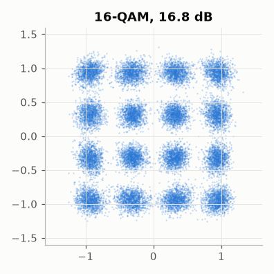
symbol rate 270.001 kBd (true 270), offset 2.700 kHz (true 2.7)
modulation 16-QAM (annotation 16-QAM), SNR 16.8 dB (18 dB injected)

The SNR found is about 1 dB below the injected one: the blind chain (resampling at an estimated rate, a truncated matched filter, the loops) adds a little distortion. With a real recording the same steps apply; a multi-channel recording is read whole (an array of shape (channels, n)) or one channel at a time.