CE-OFDM receivers, spectrum and bandwidth

Four panels, each to open next to the figure of the paper it reproduces:

1. The optimum and the phase detector at \(2\pi h = 1.4\). J. Guerreiro, R. Dinis and P. Montezuma, “On the detection of CE-OFDM signals”, IEEE Commun. Lett. 20(11), 2016, show that the optimum asymptotic BER of QPSK CE-OFDM is \(Q(\sqrt{(2\pi h)^2\, 2E_b/N_0})\) (eq. (8)) while the phase detector floors once the phase leaves \((-\pi, \pi]\) (Fig. 1). M. J. López Morales, R. Dinis and A. García Armada, Proc. IEEE Globecom Workshops, 2022, reach that optimum with a GAMP receiver (Fig. 3). Their \(E_b/N_0\) axis is shifted against the 2016 letter (by 6 dB at \(2\pi b = 0.5\), 2.5 dB at 1.4), so compare the gaps, not the abscissas.

2. Low-complexity receivers at \(2\pi h = 0.7\). A. U. Ahmed and J. R. Zeidler, “Novel low-complexity receivers for constant envelope OFDM”, IEEE Trans. Signal Process. 63(17), 2015, replace the arctangent by \(\operatorname{Im} r\) (basic linear receiver) or \(\operatorname{Im} r\,(2 - \operatorname{Re} r)\) (enhanced receiver), Fig. 6 with \(N = 64\) and 2X sampling. The lines are the library’s Bussgang analysis (CeOfdm.ber_receiver), the markers the simulation.

3. Bandwidth. R. A. Pacheco and D. Hatzinakos, Proc. IEEE ICASSP, 2006, Fig. 1: the 99 % bandwidth of a carrier phase-modulated by a flat Gaussian message (pm_occupied_bandwidth) against that of simulated CE-OFDM with 104 subcarriers.

4. Spectrum. J. Guerreiro, R. Dinis and P. Montezuma, Proc. IEEE VTC Fall, 2015, Fig. 3: the spectrum at \(2\pi h = 2\) with \(N = 128\) and \(M = 4\), from the powers \(P_i = e^{-\varphi^2}\varphi^{2i}/i!\) of the intermodulation products (CeOfdm.psd), against the mean periodogram of simulated blocks.

validation/tests/multicarrier/ce_ofdm.rs checks the same comparisons with tolerances.

import matplotlib.pyplot as plt
import numpy as np

import comnum
from comnum.plot import MUTED

TAU = 2 * np.pi
QPSK = comnum.Constellation("qam", 4).normalized()


def ber(e, d):
    wrong = np.bitwise_xor(QPSK.decide(e), QPSK.decide(d))
    return float(sum(bin(int(v)).count("1") for v in wrong)) / (2 * d.size)


def link(ce, ebn0_db, blocks, seed):
    rng = comnum.Rng(seed)
    _, d = comnum.symbols(QPSK, ce.n_subcarriers * blocks, rng)
    sigma2 = ce.noise_variance(ebn0_db + comnum.lin2db(2))
    s = ce.modulate(d)
    return d, s + rng.complex_noise(s.size, sigma2), sigma2


fig, axes = plt.subplots(2, 2, figsize=(11, 8.2))

# 1. 2πh = 1.4: phase detector, GAMP and the optimum
ax = axes[0, 0]
ce = comnum.CeOfdm(511, h=1.4 / TAU, oversampling=4)
ebn0 = np.arange(0.0, 7.0, 1.0)
pd, gamp = [], []
for i, e in enumerate(ebn0):
    d, r, s2 = link(ce, e, 30, i)
    pd.append(ber(ce.demodulate(r), d))
    gamp.append(ber(ce.gamp(r, s2, QPSK), d))
fine = np.linspace(0, 8, 81)
ax.semilogy(
    fine, comnum.theory_ce_ofdm_ber_optimum(1.4, fine), color=MUTED, label="optimum, eq. (8)"
)
ax.semilogy(ebn0, pd, "o--", label="phase detector")
ax.semilogy(ebn0, np.maximum(gamp, 1e-6), "s-", label="GAMP")
ax.set(
    ylim=(1e-5, 0.5),
    xlabel="$E_b/N_0$ (dB)",
    ylabel="BER",
    title="QPSK, $2\\pi h$ = 1.4, N = 1024 (K = 511), M = 4",
)
ax.legend(loc="lower left")

# 2. 2πh = 0.7: arctangent, basic linear and enhanced receivers
ax = axes[0, 1]
ce = comnum.CeOfdm(32, h=0.7 / TAU, oversampling=2)
ebn0 = np.arange(0.0, 15.0, 2.0)
fine = np.linspace(0, 14, 57)
names = {"arctangent": "arctangent", "linear": "basic linear", "enhanced": "enhanced"}
for j, (receiver, label) in enumerate(names.items()):
    sim = []
    for i, e in enumerate(ebn0):
        d, r, _ = link(ce, e, 2000, 100 + i)
        sim.append(ber(ce.demodulate(r, receiver=receiver), d))
    (line,) = ax.semilogy(ebn0, np.maximum(sim, 1e-7), "o^s"[j], label=label)
    if receiver != "arctangent":
        theory = ce.ber_receiver(4, fine + comnum.lin2db(2), receiver=receiver)
        ax.semilogy(fine, theory, color=line.get_color(), linewidth=1.2)
ax.semilogy(
    fine, ce.ber_esn0(4, fine + comnum.lin2db(2)), color=MUTED, linewidth=1.0, label="linear regime"
)
ax.set(
    ylim=(1e-5, 0.5),
    xlabel="$E_b/N_0$ (dB)",
    ylabel="BER",
    title="QPSK, $2\\pi h$ = 0.7, K = 32, J = 2",
)
ax.legend(loc="lower left")

# 3. the 99 % bandwidth against σ
ax = axes[1, 0]
sigmas = np.linspace(0.05, 3.0, 60)
ax.plot(sigmas, [comnum.pm_occupied_bandwidth(s) for s in sigmas], color=MUTED, label="analysis")
points = []
for sigma in [0.25, 0.5, 1.0, 1.5, 2.0, 2.5, 3.0]:
    ce = comnum.CeOfdm(104, h=sigma / TAU, oversampling=8)
    n = ce.n_fft
    _, d = comnum.symbols(QPSK, 104 * 200, comnum.Rng(3))
    blocks = ce.modulate(d).reshape(-1, n)
    p = (np.abs(np.fft.fft(blocks, axis=1)) ** 2).mean(axis=0)
    total, inside, z = p[1:].sum(), 0.0, 0
    while inside < 0.99 * total:
        z += 1
        inside += p[z] + p[n - z]
    points.append((sigma, z / 104))
ax.plot(*zip(*points, strict=True), "o", label="simulated CE-OFDM, 104 subcarriers")
ax.set(
    xlabel="$\\sigma_m$ (rad)",
    ylabel="$B_y / 2B_m$",
    title="99 % bandwidth (Pacheco & Hatzinakos 2006, Fig. 1)",
)
ax.legend(loc="upper left")

# 4. the spectrum at 2πh = 2
ax = axes[1, 1]
ce = comnum.CeOfdm(63, h=2.0 / TAU, oversampling=4)
n = ce.n_fft
_, d = comnum.symbols(QPSK, 63 * 1000, comnum.Rng(4))
blocks = ce.modulate(d).reshape(-1, n)
sim = (np.abs(np.fft.fft(blocks, axis=1)) ** 2).mean(axis=0) / n
k = np.fft.fftshift(np.fft.fftfreq(n, 1 / n)) / 64
ax.plot(k, comnum.lin2db(np.fft.fftshift(ce.psd())), color=MUTED, linewidth=1.4, label="theory")
ax.plot(k, comnum.lin2db(np.fft.fftshift(sim)), "--", linewidth=1.0, label="simulation")
ax.set(
    xlabel="$k/N$",
    ylabel="PSD (dB)",
    title="$2\\pi h$ = 2, N = 128, M = 4 (Guerreiro et al. 2015, Fig. 3)",
)
ax.legend(loc="lower center")
fig.tight_layout()

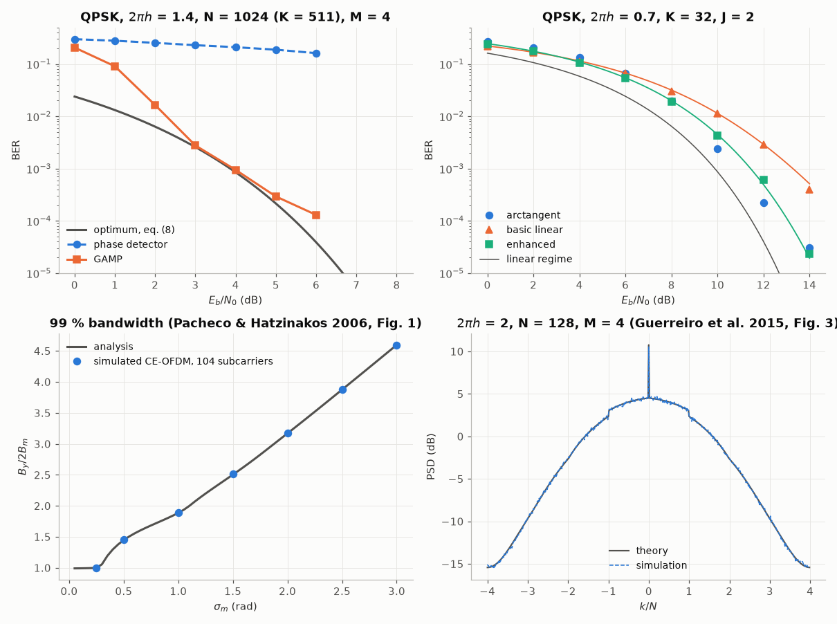
The phase detector floors at \(2\pi h = 1.4\) while GAMP follows the optimum within a fraction of a decibel, at the size of the paper (\(N = 1024\)). GAMP is a large-system algorithm: at 4 dB its BER is 1.6e-2, 4.5e-3, 1.0e-3 and 8.1e-4 for K = 63, 127, 255 and 511 data subcarriers, against 8.5e-4 for the optimum; at \(2\pi h = 0.7\) the enhanced receiver beats the basic one everywhere and the arctangent one at high BERs, as in Fig. 6 of Ahmed and Zeidler. Below \(10^{-4}\), the wraps of the phase (not unwrapped) floor the arctangent receiver.

print(f"GAMP at 6 dB: {gamp[-1]:.1e}, optimum {comnum.theory_ce_ofdm_ber_optimum(1.4, 6.0):.1e}")

GAMP at 6 dB: 1.3e-04, optimum 3.9e-05