Large MIMO: message passing (LAMA and OAMP)

With tens of streams, the maximum-likelihood search is out of reach and the linear detectors lose several dB. Approximate message passing (AMP) alternates a linear step on the whole vector and a scalar MMSE denoiser on every stream: in the large-system limit, it decouples the MIMO channel into parallel AWGN channels whose noise variance a scalar recursion, the state evolution, predicts exactly.

• LAMA (method="amp"), the complex Bayesian AMP of Jeon, Ghods, Maleki & Studer (“Optimal data detection in large MIMO”, arXiv:1811.01917, 2018), reaches the individually optimal (IO) error rate when the ratio \(\beta = n_t / n_r\) is below a threshold of the constellation (their Table II), at \(O(n_r n_t)\) per iteration. It assumes an i.i.d. Gaussian channel.

• OAMP (method="oamp"), the orthogonal AMP of Ma & Ping (IEEE Access 5, 2017), replaces the matched filter by a de-correlated LMMSE estimator: its state evolution holds for any unitarily-invariant channel, correlated ones included, at the price of an SVD of the channel.

comnum.message_passing returns the iterations of either detector, comnum.amp_state_evolution and comnum.oamp_state_evolution their predictions, and comnum.amp_thresholds the thresholds of LAMA. validation/tests/mimo/message_passing.rs checks them against both papers.

import time

import matplotlib.pyplot as plt
import numpy as np

import comnum
from comnum.plot import BACKGROUND, GREY

The thresholds of LAMA

Below \(\beta_{\min}\) the state evolution has a single fixed point and LAMA is optimal at every SNR; below \(\beta_{\max}\) it recovers the noiseless signal. Jeon et al. give them in Table II; comnum computes them from the MSE function of the denoiser.

table_ii = {"QPSK": (1.475, 2.086), "16-QAM": (0.983, 1.363), "64-QAM": (0.842, 1.157)}
print(f"{'':8s} {'βmin (paper)':>13s} {'βmin':>8s} {'βmax (paper)':>13s} {'βmax':>8s}")
for name, (bmin, bmax) in table_ii.items():
    m = 4 if name == "QPSK" else int(name.split("-")[0])
    t = comnum.amp_thresholds(comnum.Constellation("qam", m).normalized())
    print(f"{name:8s} {bmin:13.3f} {t['beta_min']:8.4f} {bmax:13.3f} {t['beta_max']:8.4f}")

          βmin (paper)     βmin  βmax (paper)     βmax
QPSK             1.475   1.4752         2.086   2.0854
16-QAM           0.983   0.9830         1.363   1.3629
64-QAM           0.842   0.8424         1.157   1.1573

The state evolution predicts every iteration

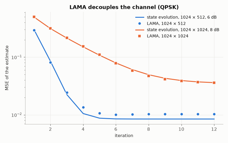
QPSK on 512 streams and 1024 receive antennas (\(\beta = 1/2\)) and on 1024 × 1024 (\(\beta = 1\)), with a channel of i.i.d. entries \(\mathcal{CN}(0, 1/n_r)\) (columns of unit norm, so that the SNR is \(\beta E_s/N_0\), Jeon et al. eq. 2). The points are the MSEs of the estimates of every iteration, averaged over six channels; the lines are the state evolution. Systems of a few hundred streams already follow it within a few percent.

qpsk = comnum.Constellation("qam", 4).normalized()
rng = comnum.Rng(7)
iterations = 12
fig, ax = plt.subplots()
for (nr, nt, snr_db), marker in zip([(1024, 512, 6.0), (1024, 1024, 8.0)], ["o", "s"], strict=True):
    beta = nt / nr
    n0 = beta / comnum.db2lin(snr_db)
    runs = []
    for _ in range(6):
        h = comnum.mimo_channel(nr, nt, rng) / np.sqrt(nr)
        x = qpsk.points[rng.integers(4, nt)]
        y = h @ x + rng.complex_noise(nr, n0)
        out = comnum.message_passing(h, y, qpsk, n0, "amp", iterations=iterations)
        runs.append(np.mean(np.abs(out["estimates"] - x) ** 2, axis=1))
    se = comnum.amp_state_evolution(qpsk, beta, n0, iterations)
    t = np.arange(1, iterations + 1)
    (line,) = ax.semilogy(t, se["mse"], label=f"state evolution, {nr} × {nt}, {snr_db:.0f} dB")
    ax.semilogy(t, np.mean(runs, axis=0), marker, color=line.get_color(), markeredgecolor=BACKGROUND,
                label=f"LAMA, {nr} × {nt}")  # fmt: skip
ax.set(xlabel="iteration", ylabel="MSE of the estimate", title="LAMA decouples the channel (QPSK)")
ax.legend()
fig.tight_layout()

Error rates: 128 receive antennas, 64 streams, 16-QAM

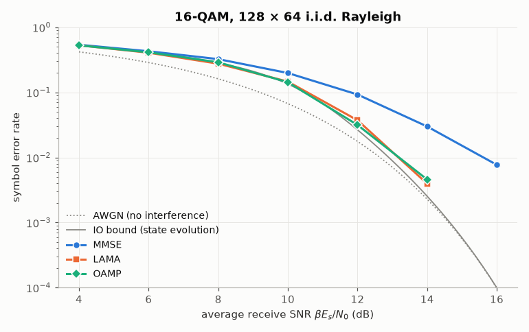
The setting of Jeon et al., Fig. 6(a): \(\beta = 1/2 < \beta_{\min}\), so the state evolution at its fixed point is the IO bound. LAMA and OAMP run 8 iterations.

q16 = comnum.Constellation("qam", 16).normalized()
nr, nt = 128, 64
beta = nt / nr


def ser(method, snr_db, n_vectors=150, correlation=0.0):
    """Symbol error rate of a detector, and its measured time per received vector."""
    n0 = beta / comnum.db2lin(snr_db)
    h = comnum.mimo_channels(
        n_vectors, nr, nt, rng, rx_correlation=correlation, tx_correlation=correlation
    ) / np.sqrt(nr)
    idx = rng.integers(16, n_vectors * nt).reshape(n_vectors, nt).T  # (n_tx, n)
    noise = rng.complex_noise(n_vectors * nr, n0).reshape(n_vectors, nr).T
    y = np.einsum("nij,jn->in", h, q16.points[idx]) + noise  # (n_rx, n)
    t0 = time.perf_counter()
    d = comnum.mimo_detect(h, y, q16, n0, method, iterations=8)
    return np.mean(d != idx), (time.perf_counter() - t0) / n_vectors


def theory_ser(s2):
    """SER of unit-energy 16-QAM in complex Gaussian noise of variance ``s2``."""
    return comnum.theory_ser(16, comnum.lin2db(1 / (4 * s2)), "qam")


snrs = np.arange(4.0, 17.0, 2.0)
curves = {
    name: [ser(m, s)[0] for s in snrs]
    for name, m in [("MMSE", "mmse"), ("LAMA", "amp"), ("OAMP", "oamp")]
}
fine = np.linspace(4, 16, 61)
io = [
    theory_ser(comnum.amp_state_evolution(q16, beta, beta / comnum.db2lin(s), 300)["noise_var"][-1])
    for s in fine
]
awgn = [theory_ser(beta / comnum.db2lin(s)) for s in fine]

fig, ax = plt.subplots()
ax.semilogy(fine, awgn, color=GREY, linestyle=":", linewidth=1.2, label="AWGN (no interference)")
ax.semilogy(fine, io, color=GREY, linewidth=1.2, label="IO bound (state evolution)")
for (name, values), marker in zip(curves.items(), ["o", "s", "D"], strict=True):
    v = np.array(values)
    keep = v > 0
    ax.semilogy(snrs[keep], v[keep], marker=marker, markeredgecolor=BACKGROUND, label=name)
ax.set(
    ylim=(1e-4, 1),
    xlabel=r"average receive SNR $\beta E_s/N_0$ (dB)",
    ylabel="symbol error rate",
    title=f"16-QAM, {nr} × {nt} i.i.d. Rayleigh",
)
ax.legend()
fig.tight_layout()

A correlated channel: where OAMP is needed

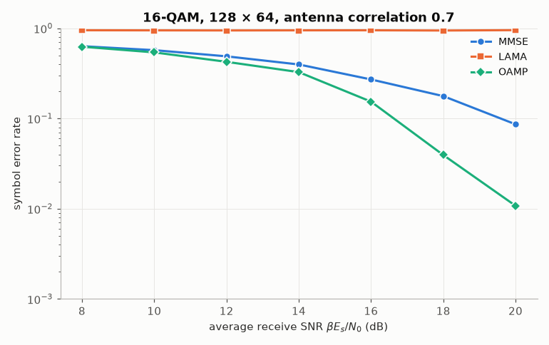
With an exponential correlation of 0.7 between adjacent antennas at both ends, the channel is no longer i.i.d.: LAMA diverges, while OAMP, whose linear step is de-correlated, keeps its advantage over MMSE.

curves = {
    name: [ser(m, s, 100, 0.7)[0] for s in snrs + 4]
    for name, m in [("MMSE", "mmse"), ("LAMA", "amp"), ("OAMP", "oamp")]
}
fig, ax = plt.subplots()
for (name, values), marker in zip(curves.items(), ["o", "s", "D"], strict=True):
    v = np.array(values)
    keep = v > 0
    ax.semilogy((snrs + 4)[keep], v[keep], marker=marker, markeredgecolor=BACKGROUND, label=name)
ax.set(
    ylim=(1e-3, 1),
    xlabel=r"average receive SNR $\beta E_s/N_0$ (dB)",
    ylabel="symbol error rate",
    title=f"16-QAM, {nr} × {nt}, antenna correlation 0.7",
)
ax.legend()
fig.tight_layout()

Computational cost

Measured time per received vector (comnum on one thread, on the machine that built this page), with \(n_r = 2 n_t\). MMSE inverts an \(n_t \times n_t\) matrix, \(O(n_t^3)\); LAMA costs \(O(n_r n_t)\) per iteration, so its 8 iterations grow as \(n_t^2\); OAMP adds an SVD of the channel, \(O(n_r n_t^2)\) once.

sizes = [8, 16, 32, 64, 128]
cost = {name: [] for name in ["MMSE", "LAMA", "OAMP"]}
for nt_ in sizes:
    nr_ = 2 * nt_
    h = comnum.mimo_channels(40, nr_, nt_, rng) / np.sqrt(nr_)
    y = np.einsum("nij,jn->in", h, q16.points[rng.integers(16, 40 * nt_).reshape(40, nt_).T])
    for name, m in [("MMSE", "mmse"), ("LAMA", "amp"), ("OAMP", "oamp")]:
        best = np.inf
        for _ in range(3):
            t0 = time.perf_counter()
            comnum.mimo_detect(h, y, q16, 0.01, m, iterations=8)
            best = min(best, (time.perf_counter() - t0) / 40)
        cost[name].append(best)

fig, ax = plt.subplots()
for (name, values), marker in zip(cost.items(), ["o", "s", "D"], strict=True):
    ax.loglog(sizes, 1e6 * np.array(values), marker=marker, markeredgecolor=BACKGROUND, label=name)
ax.set(
    xlabel="streams $n_t$ ($n_r = 2 n_t$)",
    ylabel="measured time per vector (µs)",
    title="16-QAM: time per received vector",
)
ax.legend()
fig.tight_layout()

print(f"{'streams':8s}" + "".join(f"{n:>10d}" for n in sizes))
for name, values in cost.items():
    print(f"{name:8s}" + "".join(f"{1e6 * v:10.1f}" for v in values))

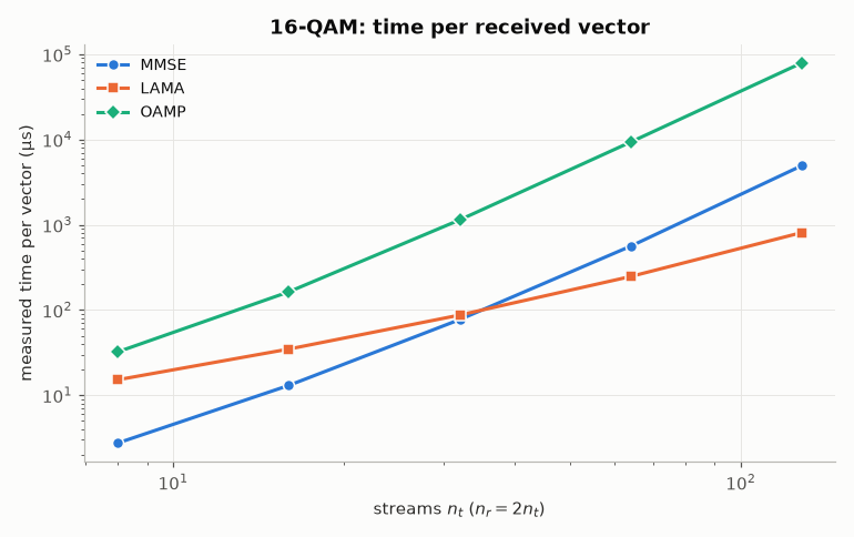
streams          8        16        32        64       128
MMSE           3.3      15.7      95.5     687.0    5565.6
LAMA          18.0      40.0     100.5     280.0     943.6
OAMP          40.8     214.4    1548.8   12723.1  107621.1