MIMO detection: linear, successive cancellation and maximum likelihood

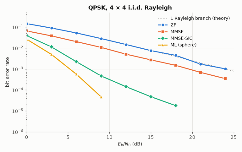
Four QPSK streams sent from four antennas and received on four, over i.i.d. Rayleigh fading with a new channel for every vector: \(y = H x + w\). The detectors trade complexity for diversity:

• ZF inverts the channel and enhances the noise: diversity \(n_r - n_t + 1 = 1\), the slope of a single Rayleigh branch;

• MMSE balances interference and noise — better at low SNR, the same slope;

• MMSE-SIC (V-BLAST) detects the strongest stream first and subtracts it;

• ML, here by the sphere decoder (exact), reaches the full receive diversity \(n_r = 4\).

The ZF curve follows the closed form of maximal-ratio combining with one branch, \(\frac{1}{2}\bigl(1 - \sqrt{\gamma/(1 + \gamma)}\bigr)\) per bit (Gray QPSK is two BPSK).

import time

import matplotlib.pyplot as plt
import numpy as np

import comnum
from comnum.plot import BACKGROUND, GREY

NR = NT = 4
c = comnum.Constellation("qam", 4).normalized()
k = c.bits_per_symbol
points = np.arange(0.0, 26.0, 3.0)
methods = {"ZF": "zf", "MMSE": "mmse", "MMSE-SIC": "mmse_sic", "ML (sphere)": "sphere"}
ber = {name: [] for name in methods}
for i, eb in enumerate(points):
    s2 = 1 / (k * comnum.db2lin(eb))  # unit energy per stream: Es/N0 = k Eb/N0
    for name, m in methods.items():
        errors = total = t = 0
        while errors < 200 and total < 4e6:
            rng = comnum.Rng.stream(9, m, i, t)
            n = 20_000
            h = comnum.mimo_channels(n, NR, NT, rng)
            idx = rng.integers(4, n * NT).reshape(n, NT).T  # (n_tx, n): stream-major
            noise = rng.complex_noise(n * NR, s2).reshape(n, NR).T
            y = np.einsum("nij,jn->in", h, c.points[idx]) + noise  # (n_rx, n)
            d = comnum.mimo_detect(h, y, c, s2, m)  # (n_tx, n)
            errors += int(np.unpackbits((d ^ idx).astype(np.uint8)[..., None], axis=-1).sum())
            total += idx.size * k
            t += 1
        # a point needs enough errors to be drawn
        ber[name].append(errors / total if errors >= 50 else np.nan)

fig, ax = plt.subplots()
eb = np.linspace(0, 25, 251)
ax.semilogy(
    eb,
    comnum.theory_ber_rayleigh_mrc(eb, branches=1),
    color=GREY,
    linewidth=1.2,
    linestyle=":",
    label="1 Rayleigh branch (theory)",
)
for (name, values), marker in zip(ber.items(), ["o", "s", "D", "^"], strict=True):
    v = np.array(values)
    keep = v > 0  # NaN (too few errors) compares false
    ax.semilogy(points[keep], v[keep], marker=marker, markeredgecolor=BACKGROUND, label=name)
ax.set(
    ylim=(1e-6, 0.5),
    xlim=(0, 25),
    xlabel="$E_b/N_0$ (dB)",
    ylabel="bit error rate",
    title=f"QPSK, {NT} × {NR} i.i.d. Rayleigh",
)
ax.legend()
fig.tight_layout()

Soft outputs feed a channel decoder: the max-log LLRs of the ML detector, and the per-stream LLRs after the unbiased MMSE filter.

rng = comnum.Rng(1)
h = comnum.mimo_channel(NR, NT, rng)
x = c.points[[0, 1, 2, 3]]
y = h @ x + rng.complex_noise(NR, 0.05)
print("ML   LLRs:", np.round(comnum.mimo_llr(h, y, c, 0.05, "ml"), 1))
print("MMSE LLRs:", np.round(comnum.mimo_llr(h, y, c, 0.05, "mmse"), 1))

ML   LLRs: [ 137.1  154.8  109.5 -156.  -156.   240.3  -67.3  -66. ]
MMSE LLRs: [ 69.2  81.4  36.8 -47.  -93.1 122.2 -31.2 -36.3]

Computational complexity

The detectors that reach the full diversity pay for it in computation. Per received vector, with a new channel every time:

Detector	Operations per vector	Behaviour
ZF, MMSE	\(O(n_t^3)\) (one inversion)	independent of the SNR
MMSE-SIC	\(O(n_t^4)\) (\(n_t\) inversions of decreasing size)	independent of the SNR
K-best	\(O(K M n_t^2)\) and a sort of \(K M\) paths per level	fixed, set by \(K\) (8 here)
Sphere	a QR, then the visited nodes	exact ML; few nodes at high SNR, many more at low SNR and for large \(M\) and \(n_t\)
ML (exhaustive)	\(O(M^{n_t} n_r n_t)\)	independent of the SNR

The expected number of nodes of the sphere decoder is polynomial in \(n_t\) over a range of high SNR (Hassibi & Vikalo, IEEE Trans. Signal Process. 53(8), 2005), but it grows exponentially with \(n_t\) at any fixed SNR (Jaldén & Ottersten, IEEE Trans. Signal Process. 53(4), 2005). The times below are measured: comnum on one thread, on the machine that built this page, best of three runs on the same vectors. Their ratios carry over to other machines, not their values. The exhaustive search of comnum evaluates \(\lVert y - H x \rVert^2\) from scratch for every hypothesis, which gives its \(M^{n_t} n_r n_t\) cost directly.

timed = {
    "ZF": "zf",
    "MMSE": "mmse",
    "MMSE-SIC": "mmse_sic",
    "K-best (K = 8)": "kbest",
    "sphere": "sphere",
    "ML (exhaustive)": "ml",
}
markers = ["o", "s", "D", "v", "^", "P"]


def time_per_vector(method, const, n_ant, eb_db, n_vectors, seed=3):
    """Measured time of the detector per received vector (seconds), best of three."""
    rng = comnum.Rng(seed)
    m = const.order
    s2 = 1 / (const.bits_per_symbol * comnum.db2lin(eb_db))
    h = comnum.mimo_channels(n_vectors, n_ant, n_ant, rng)
    idx = rng.integers(m, n_vectors * n_ant).reshape(n_vectors, n_ant).T
    noise = rng.complex_noise(n_vectors * n_ant, s2).reshape(n_vectors, n_ant).T
    y = np.einsum("nij,jn->in", h, const.points[idx]) + noise
    best = np.inf
    for _ in range(3):
        t0 = time.perf_counter()
        comnum.mimo_detect(h, y, const, s2, method)
        best = min(best, time.perf_counter() - t0)
    return best / n_vectors


snrs = np.arange(0.0, 26.0, 5.0)
per_snr = {name: [time_per_vector(m, c, 4, e, 2000) for e in snrs] for name, m in timed.items()}

fig, ax = plt.subplots()
for (name, values), marker in zip(per_snr.items(), markers, strict=True):
    ax.semilogy(snrs, 1e6 * np.array(values), marker=marker, markeredgecolor=BACKGROUND, label=name)
ax.set(
    xlabel="$E_b/N_0$ (dB)",
    ylabel="measured time per vector (µs)",
    title=f"QPSK, {NT} × {NR}: time per received vector",
)
ax.legend(ncols=2)
fig.tight_layout()

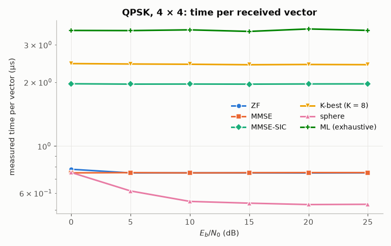
With QPSK the tree of the sphere decoder has four branches per level: it stays as cheap as a linear detector (ZF and MMSE overlap), and gets cheaper as the SNR rises. Its cost shows with a larger constellation, at low SNR, as the number of antennas grows: 16-QAM at \(E_b/N_0\) = 0 dB, from 2 × 2 to 8 × 8. The exhaustive search stops at 5 × 5 (\(16^5\) hypotheses per vector).

q16 = comnum.Constellation("qam", 16).normalized()
antennas = np.arange(2, 9)
per_size = {}
for name, m in timed.items():
    sizes = antennas[antennas <= 5] if m == "ml" else antennas
    # fewer vectors where a vector costs more: every point takes about a second at most
    count = [max(10, 2000 // 16 ** max(n - 3, 0)) if m == "ml" else 2000 for n in sizes]
    per_size[name] = (
        sizes,
        [time_per_vector(m, q16, n, 0.0, v) for n, v in zip(sizes, count, strict=True)],
    )

fig, ax = plt.subplots()
for (name, (sizes, values)), marker in zip(per_size.items(), markers, strict=True):
    ax.semilogy(
        sizes, 1e6 * np.array(values), marker=marker, markeredgecolor=BACKGROUND, label=name
    )
ax.set(
    xlabel="antennas $n_t = n_r$",
    ylabel="measured time per vector (µs)",
    title="16-QAM at $E_b/N_0$ = 0 dB: time per received vector",
    ylim=(0.2, 1e6),
)
ax.legend(ncols=2, loc="upper left")
fig.tight_layout()

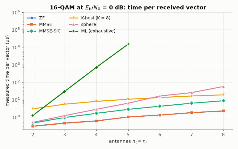
The measured times (µs per received vector):

print(f"{'detector':16s}" + "".join(f"{f'{n} × {n}':>11s}" for n in antennas))
for name, (sizes, values) in per_size.items():
    cells = dict(zip(sizes, values, strict=True))
    row = "".join(f"{1e6 * cells[n]:11.1f}" if n in cells else f"{'—':>11s}" for n in antennas)
    print(f"{name:16s}{row}")

detector              2 × 2      3 × 3      4 × 4      5 × 5      6 × 6      7 × 7      8 × 8
ZF                      0.4        0.6        0.8        1.3        1.6        2.2        2.7
MMSE                    0.4        0.6        0.8        1.3        1.6        2.2        2.7
MMSE-SIC                0.6        1.2        2.0        3.3        4.9        7.3       10.1
K-best (K = 8)          3.8        7.0       10.2       13.3       16.6       19.9       23.4
sphere                  0.6        1.6        3.7        8.2       20.9       32.5       73.1
ML (exhaustive)         1.3       31.1      811.0    19217.1          —          —          —