Raman amplification: pumps, gain flattening and the hybrid link

The pumps of a distributed Raman amplifier transfer their power to the signals about 13 THz below them, all along the span. comnum.raman_profile() solves the coupled power equations of stimulated Raman scattering (Bromage 2004) for the signals and any number of co- and counter-propagating pumps, with the measured gain spectrum of standard single-mode fibre.

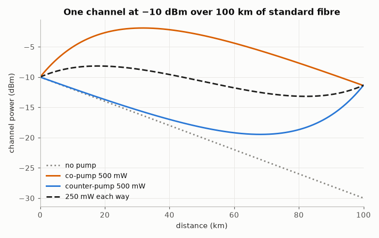
Power profiles. One channel at −10 dBm over 100 km. Without pump the power decays by 0.2 dB/km. A co-propagating pump amplifies the beginning of the span, where the signal is strong, and a counter-propagating pump amplifies the end, where it is weak. The counter-pump therefore keeps the signal away from both the high powers of the nonlinear regime and the low powers of the noise.

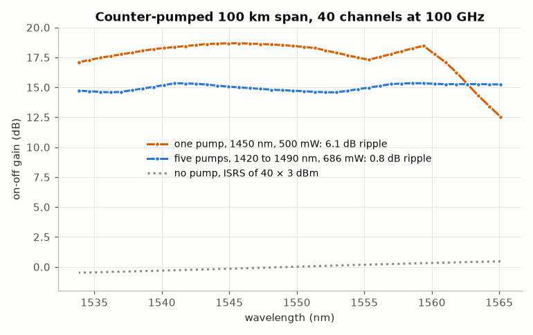
Gain flattening. A single pump gives the shape of the Raman gain: 6 dB of ripple over the C band. Five counter-pumps from 1420 to 1490 nm, whose gain spectra overlap, give 15 dB of on-off gain within 0.8 dB over 40 channels. The pumps also amplify each other: the shortest ones feed the longest ones. Without pump, inter-channel stimulated Raman scattering alone tilts a wide WDM spectrum: the high-frequency channels feed the low-frequency ones.

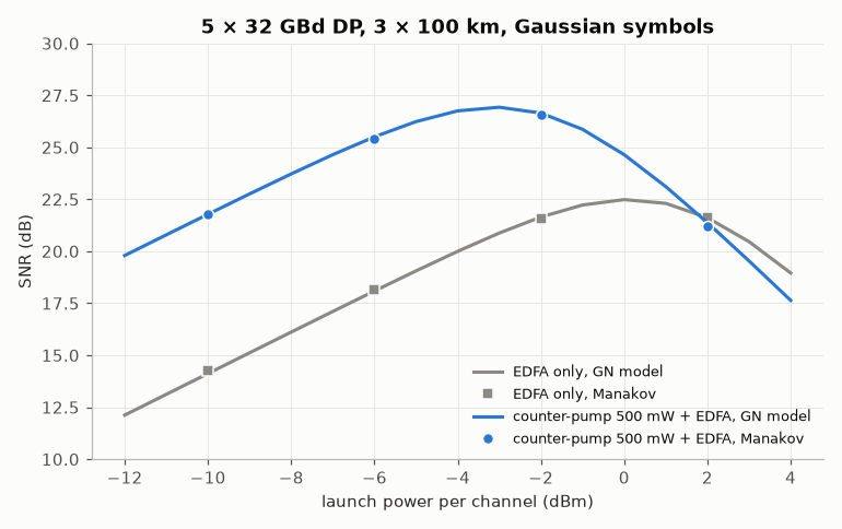
The hybrid link. Five channels over three spans of 100 km. An EDFA with an ideal gain-flattening filter restores every channel after each span, with or without a counter-pump of 500 mW at 1450 nm. The pump compensates 18.5 of the 20 dB of loss of the span, so the noise falls by 7.7 dB. It also raises the power at the end of the span, so the nonlinear interference grows and the optimal launch power drops by 3.2 dB. The optimal SNR still gains 4.4 dB. Gaussian symbols simulated by the Manakov equation with the power profiles of the spans follow the GN model with the same profiles (specs/raman_wdm.yaml, within 0.21 dB). tests/oracle/test_gnpy_oracle.py checks the profiles, the noise and the nonlinear interference against GNPy.

import matplotlib.pyplot as plt
import numpy as np
from _gallery_utils import SPECS

import comnum
from comnum.plot import BACKGROUND, BLUE, GREY, INK, RUST

The power of one channel along a span of 100 km, by direction of pumping.

span = comnum.FiberParams(span_km=100)
cases = [
    ("no pump", [], GREY, ":"),
    (
        "co-pump 500 mW",
        [{"wavelength_nm": 1450, "power_mw": 500, "direction": "co"}],
        RUST,
        "-",
    ),
    (
        "counter-pump 500 mW",
        [{"wavelength_nm": 1450, "power_mw": 500, "direction": "counter"}],
        BLUE,
        "-",
    ),
    (
        "250 mW each way",
        [
            {"wavelength_nm": 1450, "power_mw": 250, "direction": "co"},
            {"wavelength_nm": 1450, "power_mw": 250, "direction": "counter"},
        ],
        INK,
        "--",
    ),
]
fig, ax = plt.subplots()
for label, pumps, color, style in cases:
    p = comnum.raman_profile(span, [0.0], -10.0, {"pumps": pumps})
    ax.plot(p["z_km"], p["power_dbm"][0], style, color=color, label=label)
ax.set(xlabel="distance (km)", ylabel="channel power (dBm)", xlim=(0, 100),
       title="One channel at −10 dBm over 100 km of standard fibre")  # fmt: skip
ax.legend(loc="lower left")
fig.tight_layout()

On-off gain over the C band: one pump against five, and the ISRS tilt without pump.

c_band = comnum.FiberParams(span_km=100, fc_hz=193.5e12)
rel = list(np.arange(-20, 20) * 100e9 + 50e9)
wavelengths = 299_792_458.0 / (193.5e12 + np.array(rel)) * 1e9
one = [{"wavelength_nm": 1450, "power_mw": 500, "direction": "counter"}]
five = [
    {"wavelength_nm": w, "power_mw": p, "direction": "counter"}
    for w, p in [(1420, 209), (1434, 188), (1448, 85), (1462, 90), (1490, 114)]
]
fig, ax = plt.subplots()
for label, pumps, color in [("one pump, 1450 nm, 500 mW", one, RUST),
                            ("five pumps, 1420 to 1490 nm, 686 mW", five, BLUE)]:  # fmt: skip
    p = comnum.raman_profile(c_band, rel, -3.0, {"pumps": pumps, "step_km": 0.5})
    ax.plot(wavelengths, p["on_off_gain_db"], marker="o", markersize=4, markeredgecolor=BACKGROUND,
            color=color, label=f"{label}: {np.ptp(p['on_off_gain_db']):.1f} dB ripple")  # fmt: skip
p = comnum.raman_profile(c_band, rel, 3.0, {"pumps": []})
ax.plot(wavelengths, p["on_off_gain_db"], color=GREY, linestyle=":",
        label="no pump, ISRS of 40 × 3 dBm")  # fmt: skip
ax.set(xlabel="wavelength (nm)", ylabel="on-off gain (dB)", ylim=(-2, 20),
       title="Counter-pumped 100 km span, 40 channels at 100 GHz")  # fmt: skip
ax.legend(loc="center")
fig.tight_layout()

The SNR of the centre channel of the hybrid link against the launch power, simulated and GN model with the Raman power profiles.

link = comnum.Chain.from_spec(SPECS / "raman_wdm.yaml")
powers = [-10.0, -6.0, -2.0, 2.0]
res = link.run(grid={"pump_mw": [0.0, 500.0], "power_dbm": powers}, stop={"max_trials": 4})
fine = np.linspace(-12, 4, 17)
freqs = comnum.wdm_grid(5, 50e9)
fiber = comnum.FiberParams(
    n_spans=3, span_km=100, alpha_db_km=0.2, d_ps_nm_km=16, gamma_w_km=1.3, nf_db=5
)
fig, ax = plt.subplots()
for pump, color, marker, label in [(0.0, GREY, "s", "EDFA only"),
                                   (500.0, BLUE, "o", "counter-pump 500 mW + EDFA")]:  # fmt: skip
    raman = {"pumps": [{"wavelength_nm": 1450, "power_mw": pump, "direction": "counter"}]}
    gn = [comnum.gn_model(fiber, freqs, p, 32e9, rolloff=0.1, raman=raman)["snr_db"] for p in fine]
    ax.plot(fine, gn, color=color, label=f"{label}, GN model")
    _, snr = res.series("power_dbm", "snr_db", pump_mw=pump)
    ax.plot(powers, snr, marker=marker, linestyle="none", color=color, markeredgecolor=BACKGROUND,
            label=f"{label}, Manakov")  # fmt: skip
ax.set(xlabel="launch power per channel (dBm)", ylabel="SNR (dB)", ylim=(10, 30),
       title="5 × 32 GBd DP, 3 × 100 km, Gaussian symbols")  # fmt: skip
ax.legend(loc="lower right", fontsize="small")
fig.tight_layout()