The LoRa modulation: error rates, spectrum and interference

Chirp spread spectrum, the modulation of LoRa (comnum.Css), in four panels, each to open next to the figure of the paper it reproduces. The SNR is that of a sample at one sample per chip, the abscissa of the papers.

1. Error rate over AWGN. O. Afisiadis, M. Cotting, A. Burg and A. Balatsoukas-Stimming, “On the error rate of the LoRa modulation with interference”, IEEE Trans. Wireless Commun. 19(2), 2020, Fig. 2: the exact SER of their eq. (16) (theory_css_ser), its approximation (17), and simulated points.

2. FSCM against FSK. L. Vangelista, “Frequency shift chirp modulation: the LoRa modulation”, IEEE Signal Process. Lett. 24(12), 2017, Fig. 1: SF 7 over AWGN, where both are orthogonal signalling, and over the channel \(\sqrt{0.8}\,\delta[n] + \sqrt{0.2}\,\delta[n-1]\), where the chirp spreads the loss over the band.

3. Spectrum. M. Chiani and A. Elzanaty, “On the LoRa modulation for IoT: waveform properties and spectral analysis”, IEEE Internet Things J. 6(5), 2019, Fig. 3a: the continuous spectrum of the complex envelope (eq. (20), Fresnel functions); lines hold exactly \(1/M\) of the power.

4. Interference. Afisiadis et al. 2020, Fig. 7: a same-SF interferer 3 dB below the signal, neither chip- nor phase-aligned; the approximation (63) with the strongest bin at \([-\lfloor\tau\rceil]_M\) (their eq. (58) prints \(\lfloor\tau\rceil\)) against a simulation.

LoRa is a trademark of Semtech; this models the published descriptions for research. validation/tests/modulation/css.rs checks the same comparisons with tolerances.

import matplotlib.pyplot as plt
import numpy as np

import comnum
from comnum.plot import MUTED


def ser_sim(css, snr_db, n, seed, taps=(1.0,)):
    rng = comnum.Rng(seed)
    sym = rng.integers(css.m, n)
    x = css.modulate(sym)
    y = np.convolve(x, np.asarray(taps))[: x.size]
    y = y + rng.complex_noise(y.size, 1 / comnum.db2lin(snr_db))
    return float(np.mean(css.demodulate(y) != sym))


fig, axes = plt.subplots(2, 2, figsize=(11, 8.2))

# 1. SER over AWGN, SF 7 to 12
ax = axes[0, 0]
for sf in range(7, 13):
    snr = np.linspace(-26, -5, 85)
    (line,) = ax.semilogy(snr, comnum.theory_css_ser(sf, snr), linewidth=1.4, label=f"SF {sf}")
    ax.semilogy(
        snr,
        comnum.theory_css_ser(sf, snr, approximation="rice"),
        ":",
        color=line.get_color(),
        linewidth=1.0,
    )
    points = np.arange(-26, -5)
    points = points[
        (comnum.theory_css_ser(sf, points * 1.0) > 3e-3)
        & (comnum.theory_css_ser(sf, points * 1.0) < 0.5)
    ]
    sim = [ser_sim(comnum.Css(sf), p, 3000 if sf < 11 else 1000, sf) for p in points]
    ax.semilogy(points, sim, "o", color=line.get_color(), markersize=4)
ax.set(
    ylim=(1e-5, 1),
    xlabel="SNR per sample (dB)",
    ylabel="SER",
    title="AWGN: exact (16), approximation (17), simulation",
)
ax.legend(loc="lower left", ncol=2, fontsize=8)

# 2. FSCM and FSK, flat and frequency-selective
ax = axes[0, 1]
snr = np.arange(-12, 0, 1.0)
flat = comnum.theory_css_ber(7, snr)
ax.semilogy(snr, flat, color=MUTED, label="flat (FSCM = FSK)")
taps = (np.sqrt(0.8), np.sqrt(0.2))
for waveform, marker in [("vangelista", "s"), ("fsk", "^")]:
    css = comnum.Css(7, waveform=waveform)
    ber = [ser_sim(css, s, 8000, 7, taps) * 128 / 254 for s in snr]
    ax.semilogy(snr, np.maximum(ber, 1e-6), marker + "-", label=f"selective, {waveform}")
ax.set(
    ylim=(1e-5, 0.5),
    xlabel="SNR per sample (dB)",
    ylabel="BER",
    title="SF 7 (Vangelista 2017, Fig. 1)",
)
ax.legend(loc="lower left")

# 3. the continuous spectrum
ax = axes[1, 0]
f = np.linspace(0, 1, 401)
for sf in (3, 5, 7):
    g = comnum.css_continuous_spectrum(sf, f)
    ax.plot(f, comnum.lin2db(np.maximum(g, 1e-12)), label=f"SF {sf}")
ax.set(
    ylim=(-50, 5),
    xlabel="$f/B$",
    ylabel="$10 \\log_{10} G^c(f) B$",
    title="Continuous spectrum (Chiani & Elzanaty 2019, Fig. 3a)",
)
ax.legend()

# 4. same-SF interference, SF 9, P_I = -3 dB
ax = axes[1, 1]
snr = np.arange(-18, -8, 1.0)
ax.semilogy(snr, comnum.theory_css_ser(9, snr), color=MUTED, linewidth=1.0, label="AWGN only")
approx = [comnum.theory_css_ser_interference(9, s, -3.0) for s in snr]
ax.semilogy(snr, approx, label="approximation (63)")
css = comnum.Css(9)
rng = comnum.Rng(9)
sim = []
for s in snr[:7:2]:
    n, errors = 4000, 0
    for _ in range(n):
        a, s1, s2 = (int(v) for v in rng.integers(512, 3))
        tau = float(rng.uniform(1)[0] * 512)
        phase = np.exp(2j * np.pi * rng.uniform(2))
        y = phase[0] * css.symbol(a) + phase[1] * 10 ** (-3 / 20) * css.interferer(s1, s2, tau)
        y = y + rng.complex_noise(512, 1 / comnum.db2lin(s))
        errors += int(css.demodulate(y)[0] != a)
    sim.append(errors / n)
ax.semilogy(snr[:7:2], np.maximum(sim, 1e-5), "o", label="simulation")
ax.set(
    ylim=(1e-5, 1),
    xlabel="SNR per sample (dB)",
    ylabel="SER",
    title="SF 9, interferer at -3 dB (Afisiadis et al. 2020, Fig. 7)",
)
ax.legend(loc="lower left")
fig.tight_layout()

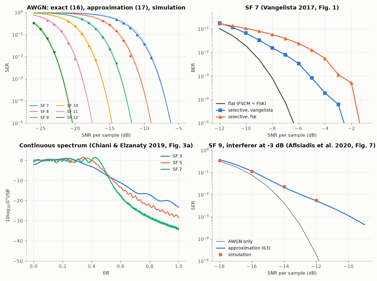
The exact SER of eq. (16) follows the simulation over the whole range and eq. (17) within 30 %. Over the frequency-selective channel the chirp loses about 1 dB where FSK loses about 4 dB; the simulated FSCM is about 0.5 dB above the curve of Vangelista’s figure, whose AWGN curve the theory reproduces exactly.

print(
    f"SF 7 at -8 dB: SER {comnum.theory_css_ser(7, -8.0):.2e} (Fig. 2 of Afisiadis et al.: 1.8e-3)"
)

SF 7 at -8 dB: SER 1.61e-03 (Fig. 2 of Afisiadis et al.: 1.8e-3)