5G NR: numerology, synchronisation block and reference signals

NR keeps the OFDM of LTE and scales it: the subcarrier spacing is \(\Delta f = 2^{\mu} \cdot 15\) kHz, a 1 ms subframe holds \(2^{\mu}\) slots of 14 symbols, and the cyclic prefix shrinks as \(2^{-\mu}\) (X. Lin et al., “5G New Radio: Unveiling the Essentials of the Next Generation Wireless Access Technology”, IEEE Commun. Standards Mag. 3(3), 2019, Sec. II; \(\mu = 0\) is the numerology of LTE, D. Astély et al., IEEE Commun. Mag. 47(4), 2009). This page builds the pieces a receiver meets first: the numerology (comnum.nr_numerology(), comnum.nr_ofdm_modulate()), the synchronisation signal block that carries the cell identity (comnum.nr_ssb_grid(), comnum.nr_detect_cell_id()) and the demodulation reference signals of the data channel (comnum.nr_pdsch_dmrs()).

The sequences, the positions and the modulation follow TS 38.211 and agree with py3gpp, an open reimplementation of the 5G functions of MATLAB (tests/oracle/test_nr_oracle.py): bit for bit for the sequences and the positions, to 10⁻¹⁴ for the waveforms.

import matplotlib.pyplot as plt
import numpy as np
from matplotlib.colors import ListedColormap

import comnum
from comnum.plot import BLUE, CRIMSON, PAPER, SKY, TEAL

Numerology

At the sampling rate \(N_{\mathrm{FFT}} \Delta f\), the first symbol of every half subframe has a longer prefix, so that the half subframe lasts exactly 0.5 ms.

print(" mu   Δf (kHz)  slot (µs)  prefix (µs)  long prefix (µs)")
for mu in range(5):
    info = comnum.nr_numerology(mu, n_fft=4096)
    fs, cp = info["sample_rate"], info["cp_lengths"]
    slot = 1e3 / info["slots_per_subframe"]
    print(
        f"{mu:3d} {info['subcarrier_spacing_hz'] / 1e3:9.0f} {slot:10.1f} {cp[1] / fs * 1e6:12.2f} {cp[0] / fs * 1e6:17.2f}"
    )

mu   Δf (kHz)  slot (µs)  prefix (µs)  long prefix (µs)
 0        15     1000.0         4.69              5.21
 1        30      500.0         2.34              2.86
 2        60      250.0         1.17              1.69
 3       120      125.0         0.59              1.11
 4       240       62.5         0.29              0.81

The synchronisation signal block

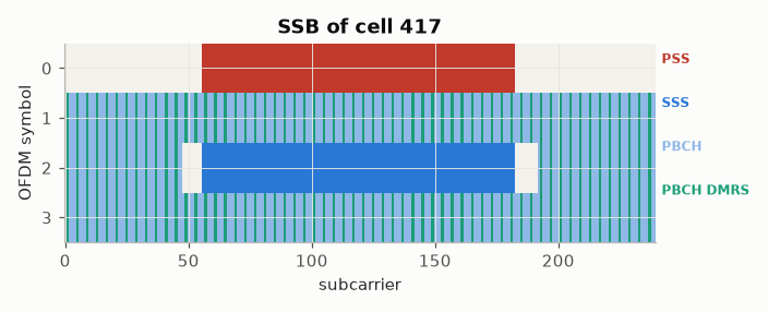
4 symbols × 240 subcarriers: the PSS (an m-sequence of length 127, one of 3), the SSS (a Gold sequence of length 127, one of 336), the broadcast channel PBCH and its DMRS on one subcarrier in four, shifted by the cell identity (Lin et al., Sec. III-A and their Fig. 2). The 1008 identities are \(3 N_{\mathrm{ID}}^{(1)} + N_{\mathrm{ID}}^{(2)}\).

cell = 417
kinds = ["pss", "sss", "pbch", "pbch_dmrs"]
layout = np.zeros((240, 4), int)  # (subcarriers, symbols)
for i, kind in enumerate(kinds, start=1):
    kl = comnum.nr_ssb_indices(cell, kind)  # (k, l) pairs
    layout[kl[:, 0], kl[:, 1]] = i
cmap = ListedColormap([PAPER, CRIMSON, BLUE, SKY, TEAL])
fig, ax = plt.subplots(figsize=(6.4, 2.6))
ax.imshow(layout.T, aspect="auto", cmap=cmap, interpolation="nearest", vmin=0, vmax=4)
ax.set(xlabel="subcarrier", ylabel="OFDM symbol", yticks=range(4), title=f"SSB of cell {cell}")
for i, (name, c) in enumerate(
    zip(["PSS", "SSS", "PBCH", "PBCH DMRS"], cmap.colors[1:], strict=True)
):
    ax.text(1.01, 0.9 - 0.22 * i, name, color=c, transform=ax.transAxes, fontsize=8, weight="bold")
fig.tight_layout()

Cell search

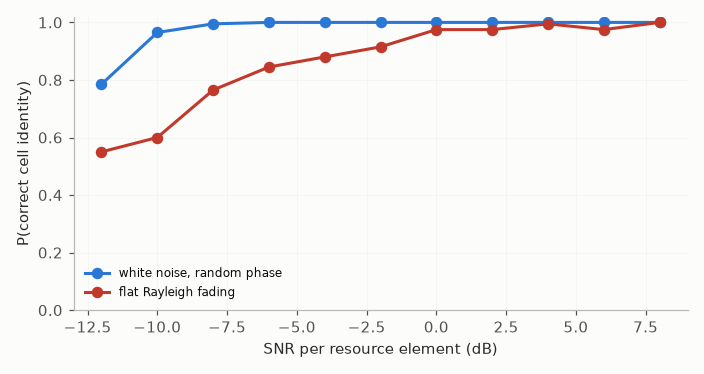
The PSS is found by correlation with the three candidates; the channel, assumed flat, is estimated on it; the SSS is then correlated coherently with the 336 candidates of that PSS. The 127 subcarriers of each sequence give 21 dB of correlation gain: with white noise and a random phase the identity is found down to -8 dB per resource element. Over a flat Rayleigh channel the failures come from the fades, whose probability falls only as 1/SNR (one branch of diversity): the reason why a terminal combines several SSBs of a burst before it decides.

rng = comnum.Rng(30)
snrs = np.arange(-12.0, 9.0, 2.0)
trials = 200
fig, ax = plt.subplots(figsize=(6.4, 3.4))
for fading, color, label in [
    (False, BLUE, "white noise, random phase"),
    (True, CRIMSON, "flat Rayleigh fading"),
]:
    p_ok = []
    for snr in snrs:
        ok = 0
        for _ in range(trials):
            cid = int(rng.integers(1008, 1)[0])
            h = rng.complex_noise(1, 1.0)[0] if fading else np.exp(2j * np.pi * rng.uniform(1)[0])
            noise = rng.complex_noise(960, comnum.db2lin(-snr)).reshape(4, 240).T
            y = h * comnum.nr_ssb_grid(cid) + noise  # the (240, 4) grid
            ok += comnum.nr_detect_cell_id(y)[0] == cid
        p_ok.append(ok / trials)
    ax.plot(snrs, p_ok, "o-", color=color, label=label)
ax.set(xlabel="SNR per resource element (dB)", ylabel="P(correct cell identity)", ylim=(0, 1.02))
ax.grid(alpha=0.3)
ax.legend(fontsize=8)
fig.tight_layout()

Demodulation reference signals of the PDSCH

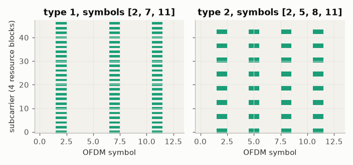
Front-loaded (the first DMRS symbol is the third or fourth of the slot), with up to three additional symbols for mobility, on one subcarrier in two (configuration type 1) or two in six (type 2), QPSK of the Gold sequence of 3GPP (Lin et al., Sec. VI-A). pilot_table of the Rust module hands them to the channel estimators of comnum_waveform::ofdm::estimation.

fig, axes = plt.subplots(1, 2, figsize=(6.4, 3.0), sharey=True)
for ax, (ctype, add) in zip(axes, [(1, 2), (2, 3)], strict=True):
    d = comnum.nr_pdsch_dmrs(4, config_type=ctype, additional_position=add, n_id=cell)
    m = np.zeros((48, 14))  # (subcarriers, symbols)
    m[d["indices"][:, 0], d["indices"][:, 1]] = 1
    ax.imshow(
        m,
        aspect="auto",
        cmap=ListedColormap([PAPER, TEAL]),
        origin="lower",
    )
    ax.set(xlabel="OFDM symbol", title=f"type {ctype}, symbols {d['symbols'].tolist()}")
axes[0].set_ylabel("subcarrier (4 resource blocks)")
fig.tight_layout()

The waveform

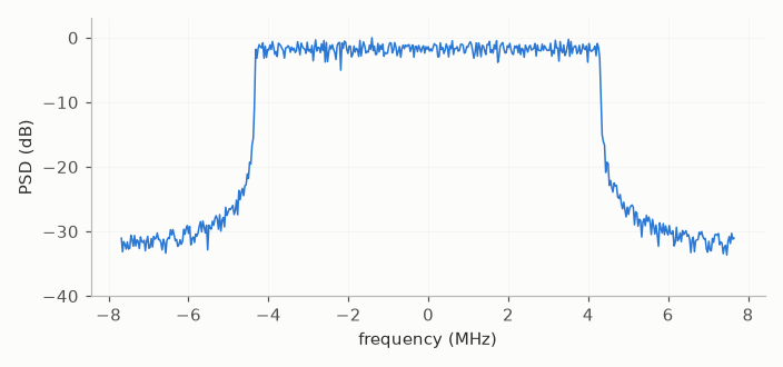
comnum.nr_ofdm_modulate() maps a grid (subcarriers × symbols) to samples with the prefixes of the numerology; here a slot at 30 kHz on 24 resource blocks: its spectrum occupies \(12 \times 24 \times 30\) kHz = 8.64 MHz.

mu, n_rb, n_fft = 1, 24, 512
k = 12 * n_rb
g = (np.sign(rng.gaussian(k * 14)) + 1j * np.sign(rng.gaussian(k * 14))).reshape(k, 14) / np.sqrt(2)
x = comnum.nr_ofdm_modulate(g, mu, n_fft)
fs = comnum.nr_numerology(mu, n_fft=n_fft)["sample_rate"]
spec = np.fft.fftshift(
    np.abs(np.fft.fft(x[: (x.size // n_fft) * n_fft].reshape(-1, n_fft), axis=1)) ** 2
).mean(0)
f = np.fft.fftshift(np.fft.fftfreq(n_fft, 1 / fs)) / 1e6
fig, ax = plt.subplots(figsize=(6.4, 3.0))
ax.plot(f, comnum.lin2db(spec / spec.max()), color=BLUE, linewidth=1)
ax.set(xlabel="frequency (MHz)", ylabel="PSD (dB)", ylim=(-40, 3))
ax.grid(alpha=0.3)
fig.tight_layout()
print(f"{x.size} samples at {fs / 1e6:.2f} MS/s: {x.size / fs * 1e3:.3f} ms")

7680 samples at 15.36 MS/s: 0.500 ms