Power amplifiers and digital predistortion

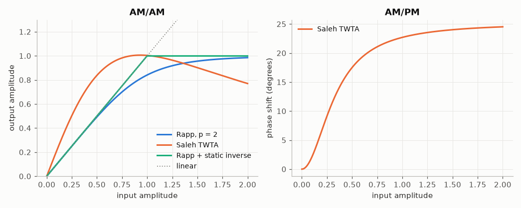
A power amplifier compresses the large amplitudes: its AM/AM (and AM/PM) conversion is linear at low power and saturates. Driven by OFDM, whose peaks are rare but high, it creates in-band distortion (EVM) and out-of-band emission (spectral regrowth, measured by the adjacent channel leakage ratio, ACLR).

• Models. Rapp’s solid-state amplifier (Proc. 2nd ECSC, 1991), Saleh’s travelling-wave tube (IEEE Trans. Commun. 29(11), 1981), and the memory-polynomial class-AB amplifier of Ding et al. (IEEE Trans. Commun. 52(1), 2004), after Kim & Konstantinou (Electron. Lett. 37(23), 2001).

• Static predistortion. For a memoryless model, the inverse AM/AM makes the cascade an ideal envelope limiter.

• Digital predistortion with memory. A memory polynomial trained by indirect learning: the post-inverse of the amplifier is fitted by least squares and copied in front of it (Eun & Powers, IEEE Trans. Signal Process. 45(1), 1997; Ding et al. 2004; Morgan et al., IEEE Trans. Signal Process. 54(10), 2006).

import matplotlib.pyplot as plt
import numpy as np

import comnum
from comnum.plot import BACKGROUND, BLUE, GREY, MUTED, ORANGE

r = np.linspace(0.0, 2.0, 400)
fig, (ax1, ax2) = plt.subplots(1, 2, figsize=(9.5, 3.8))
ax1.plot(r, np.abs(comnum.pa_rapp(r, smoothness=2.0)), label="Rapp, p = 2")
ax1.plot(r, np.abs(comnum.pa_saleh(r)), label="Saleh TWTA")
ax1.plot(
    r,
    np.abs(
        comnum.pa_rapp(comnum.rapp_predistort(r, smoothness=2.0, max_output=0.999), smoothness=2.0)
    ),
    label="Rapp + static inverse",
)
ax1.plot(r, r, color=GREY, linestyle=":", linewidth=1.2, label="linear")
ax1.set(xlabel="input amplitude", ylabel="output amplitude", title="AM/AM", ylim=(0, 1.3))
ax1.legend()
ax2.plot(r, np.degrees(np.angle(comnum.pa_saleh(r))), color=ORANGE, label="Saleh TWTA")
ax2.set(xlabel="input amplitude", ylabel="phase shift (degrees)", title="AM/PM")
ax2.legend()
fig.tight_layout()

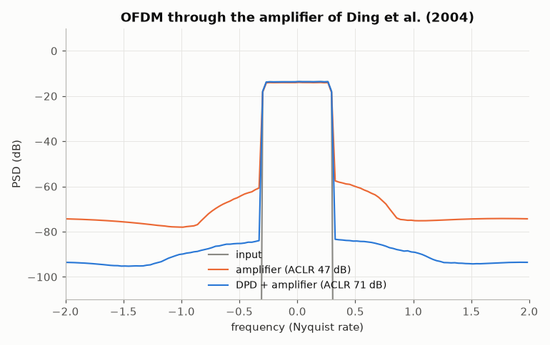
The spectrum of 16-QAM OFDM (150 of 256 subcarriers) through the memory-polynomial amplifier, with and without predistortion. The periodogram is aligned on the cyclic blocks, so the out-of-band density is the regrowth of the amplifier alone.

ofdm = comnum.Ofdm(256, 150)
c = comnum.Constellation("qam", 16).normalized()
_, d = comnum.symbols(c, 150 * 300, comnum.Rng(3))
x = 0.15 * ofdm.modulate(d)
g = 1.0513 + 0.0904j
dpd = comnum.MemoryPolynomialDpd([1, 3, 5], 3)
dpd.train_indirect(x, comnum.pa_memory_polynomial, gain=g, iterations=2)
fs, bw = 4.0, 150 / 256
signals = {
    "input": x * g,
    "amplifier": comnum.pa_memory_polynomial(x),
    "DPD + amplifier": comnum.pa_memory_polynomial(dpd.apply(x)),
}
fig, ax = plt.subplots()
for (name, y), color in zip(signals.items(), [GREY, ORANGE, BLUE], strict=True):
    f, s = comnum.periodogram(y, fs=fs, nfft=ofdm.fft_len)
    # average over 8 bins for readability
    k = 8
    f8, s8 = f.reshape(-1, k).mean(axis=1), s.reshape(-1, k).mean(axis=1)
    aclr = comnum.aclr_db(f, s, bw, bw)
    ax.plot(
        f8,
        comnum.lin2db(s8 + 1e-30),
        color=color,
        linewidth=1.4,
        label=f"{name} (ACLR {aclr:.0f} dB)" if aclr < 200 else f"{name}",
    )
ax.set(
    xlim=(-2, 2),
    ylim=(-110, 10),
    xlabel="frequency (Nyquist rate)",
    ylabel="PSD (dB)",
    title="OFDM through the amplifier of Ding et al. (2004)",
)
ax.legend(loc="lower center")
fig.tight_layout()

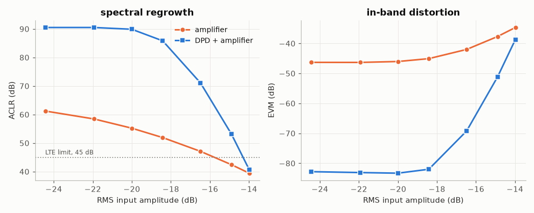
ACLR and EVM against the input back-off: the predistorted amplifier stays linear up to a much higher drive, i.e. a given ACLR is met with less back-off (more efficiency).

scales = np.array([0.06, 0.08, 0.1, 0.12, 0.15, 0.18, 0.2])


def evm_db(y, scale):
    rx = ofdm.demodulate(y / (scale * g))
    a = np.vdot(d, rx) / np.vdot(d, d)
    return comnum.lin2db(np.mean(np.abs(rx / a - d) ** 2))


res = {"amplifier": ([], []), "DPD + amplifier": ([], [])}
for s in scales:
    xs = s * ofdm.modulate(d)
    p = comnum.MemoryPolynomialDpd([1, 3, 5], 3)
    p.train_indirect(xs, comnum.pa_memory_polynomial, gain=g, iterations=2)
    for name, y in [
        ("amplifier", comnum.pa_memory_polynomial(xs)),
        ("DPD + amplifier", comnum.pa_memory_polynomial(p.apply(xs))),
    ]:
        f, sd = comnum.periodogram(y, fs=fs, nfft=ofdm.fft_len)
        res[name][0].append(min(comnum.aclr_db(f, sd, bw, bw), 120.0))
        res[name][1].append(evm_db(y, s))
drive = 20 * np.log10(scales)
fig, (ax1, ax2) = plt.subplots(1, 2, figsize=(9.5, 3.8))
for (name, (aclr, evm)), color, marker in zip(res.items(), [ORANGE, BLUE], ["o", "s"], strict=True):
    ax1.plot(drive, aclr, marker=marker, color=color, markeredgecolor=BACKGROUND, label=name)
    ax2.plot(drive, evm, marker=marker, color=color, markeredgecolor=BACKGROUND, label=name)
ax1.axhline(45, color=GREY, linestyle=":", linewidth=1.2)
ax1.text(drive[0], 46, "LTE limit, 45 dB", fontsize=8, color=MUTED)
ax1.set(xlabel="RMS input amplitude (dB)", ylabel="ACLR (dB)", title="spectral regrowth")
ax2.set(xlabel="RMS input amplitude (dB)", ylabel="EVM (dB)", title="in-band distortion")
ax1.legend()
fig.tight_layout()