Nonlinear fibre propagation and digital back-propagation

The classical launch-power sweep of a long-haul optical link: 16-QAM at 32 GBd over 10 spans of 80 km of standard single-mode fibre with an EDFA (noise figure 4.5 dB) after every span, simulated by the split-step Fourier method (1 km steps). At low power the amplified spontaneous emission limits the SNR, which grows by 1 dB per dB of launch power; at high power the Kerr nonlinearity (\(\gamma = 1.3\) /(W·km)) takes over and the SNR falls. The optimum is the maximum of this “bell”.

Dispersion compensation alone (cdc) undoes the linear part of the channel only. Digital back-propagation solves the propagation equation backwards with the coefficients negated (comnum.Ssfm.backpropagate()): with enough steps per span it removes the deterministic nonlinear distortion of a single channel, and the optimum moves to a higher power and a higher SNR (Ip & Kahn, J. Lightw. Technol. 26(20), 2008).

import matplotlib.pyplot as plt
import numpy as np

import comnum
from comnum.plot import BACKGROUND, MUTED

RS, SPS, N = 32e9, 4, 4096
FS = RS * SPS
fiber = comnum.FiberParams(n_spans=10)
link = comnum.Ssfm(fiber, step_km=1.0)
c = comnum.Constellation("qam", 16).normalized()
h = comnum.pulse_shape("rrc", SPS, n_taps=4 * 256 + 1, rolloff=0.1)
powers = np.arange(-6.0, 10.1, 2.0)
receivers = {"CDC": None, "DBP, 1 step/span": 1, "DBP, 20 steps/span": 20}


def snr_db(r, x):
    z = comnum.pnorm(comnum.downsample(comnum.fir_filter(h, r), SPS))
    return comnum.fast_ber_calc(z[256:-256], x[256:-256], c)[2]


snr = {name: [] for name in receivers}
for i, p in enumerate(powers):
    rng = comnum.Rng.stream(11, "launch-power", i, 0)
    _, x = comnum.symbols(c, N, rng)
    tx = comnum.pnorm(comnum.fir_filter(h, comnum.upsample(x, SPS))) * np.sqrt(comnum.dbm2w(p))
    y = link.propagate(tx, FS, rng=rng)
    for name, steps in receivers.items():
        r = (
            comnum.cdc(y, fiber, fiber.total_km, FS)
            if steps is None
            else link.backpropagate(y, FS, steps_per_span=steps)
        )
        snr[name].append(snr_db(r, x))

fig, ax = plt.subplots()
for (name, values), marker in zip(snr.items(), ["o", "s", "D"], strict=True):
    ax.plot(powers, values, marker=marker, markeredgecolor=BACKGROUND, label=name)
    if name != "DBP, 1 step/span":  # its optimum sits on top of the CDC one
        k = int(np.argmax(values))
        below = name == "CDC"
        ax.annotate(
            f"{values[k]:.1f} dB",
            (powers[k], values[k]),
            textcoords="offset points",
            xytext=(0, -15 if below else 8),
            ha="center",
            fontsize=8,
            color=MUTED,
        )
ax.set(
    xlabel="launch power (dBm)",
    ylabel="effective SNR (dB)",
    title="16-QAM, 32 GBd, 10 × 80 km SSMF",
)
ax.legend(loc="lower center")
fig.tight_layout()

for name, values in snr.items():
    k = int(np.argmax(values))
    print(f"{name:<20} optimum {powers[k]:+.0f} dBm, SNR {values[k]:.1f} dB")

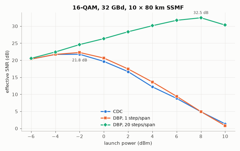
CDC                  optimum -2 dBm, SNR 21.8 dB
DBP, 1 step/span     optimum -2 dBm, SNR 22.3 dB
DBP, 20 steps/span   optimum +8 dBm, SNR 32.5 dB