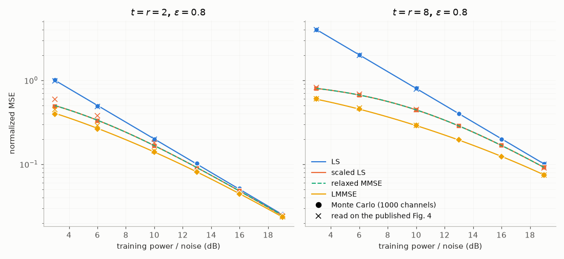
Biguesh & Gershman 2006, Fig. 4: LS, scaled LS, relaxed MMSE and LMMSE

Fig. 4 of M. Biguesh and A. B. Gershman, “Training-based MIMO channel estimation: a study of estimator tradeoffs and optimal training signals”, IEEE Trans. Signal Process. 54(3), 2006, compares four estimators of a flat \(r \times t\) channel from \(S = H P + V\), each needing more prior knowledge than the last: least squares (none), scaled LS (the trace of \(R_H = E\{H^H H\}\)), the relaxed MMSE (the same trace, \(R_H\) replaced by a scaled identity) and the LMMSE (all of \(R_H\)). The training is the DFT matrix of orthogonal rows (their eq. (10)), the transmit correlation exponential with \(\varepsilon = 0.8\) (eq. (60)), the abscissa the training power over the noise in dB.

The lines are the closed-form MSE of comnum.MimoTraining (their eqs. (12), (20), (49) and (28)); the dots a Monte Carlo of 1000 channels; the crosses the values read on the published figure. Scaled LS and relaxed MMSE coincide under orthogonal training, as eq. (48) shows. The card validation/cards/biguesh2006.yaml checks 121 readings of Figs. 1-4 within 7.4 %; for \(t = r = 2\) below 6 dB the published SLS and LMMSE markers lie 11-18 % above the paper’s own equations (left of the figure), the only points where the figure and its equations disagree.

import matplotlib.pyplot as plt
import numpy as np

import comnum
from comnum.plot import BACKGROUND

EPS, RUNS = 0.8, 1000
x_db = np.linspace(3, 19, 81)
mc_db = [3, 6, 10, 13, 16, 19]
# readings of Fig. 4 (vector paths of the figure), SLS = RMMSE
readings = {
    8: {
        "ls": [4.0, 2.0, 0.79, 0.100],
        "sls": [0.82, 0.68, 0.45, 0.091],
        "mmse": [0.60, 0.47, 0.29, 0.074],
    },
    2: {
        "ls": [0.98, 0.485, 0.20, 0.024],
        "sls": [0.59, 0.38, 0.18, 0.024],
        "mmse": [0.45, 0.29, 0.143, 0.024],
    },
}
names = {"ls": "LS", "sls": "scaled LS", "rmmse": "relaxed MMSE", "mmse": "LMMSE"}


def correlation(t, r):
    return r * comnum.exponential_correlation(t, EPS)


def monte_carlo(t, r, estimator, snr_db, rng):
    p = comnum.MimoTraining.orthogonal(t, total_power=10 ** (snr_db / 10))
    r_h, err = correlation(t, r), 0.0
    for _ in range(RUNS):
        h = comnum.mimo_channel(r, t, rng, tx_correlation=EPS)
        v = rng.complex_noise(r * t, 1.0).reshape(r, t)
        h_hat = p.estimate(h @ p.symbols + v, estimator, 1.0, r_h=r_h, trace=float(r * t))
        err += np.sum(np.abs(h - h_hat) ** 2)
    return err / RUNS / (r * t)


fig, axes = plt.subplots(1, 2, figsize=(10, 4.6), sharey=True)
rng = comnum.Rng(2006)
for ax, t in zip(axes, [2, 8], strict=True):
    r = t
    for est, marker in zip(["ls", "sls", "rmmse", "mmse"], ["o", "s", "", "D"], strict=True):
        cf = [
            comnum.MimoTraining.orthogonal(t, total_power=10 ** (x / 10)).mse(
                est, correlation(t, r), 1.0, r
            )
            / (r * t)
            for x in x_db
        ]
        style = "--" if est == "rmmse" else "-"
        (line,) = ax.semilogy(x_db, cf, style, linewidth=1.4, label=names[est])
        if est == "rmmse":
            continue
        mc = [monte_carlo(t, r, est, x, rng) for x in mc_db]
        ax.semilogy(mc_db, mc, marker, color=line.get_color(), markeredgecolor=BACKGROUND)
        ax.semilogy([3, 6, 10, 19], readings[t][est], "x", color=line.get_color(), markersize=7)
    ax.plot([], [], "ok", label="Monte Carlo (1000 channels)")
    ax.plot([], [], "xk", label="read on the published Fig. 4")
    ax.set(xlabel="training power / noise (dB)", title=f"$t = r = {t}$, $\\varepsilon = {EPS}$")
    ax.grid(True, which="both", alpha=0.3)
axes[0].set_ylabel("normalized MSE")
axes[1].legend(loc="lower left")
fig.tight_layout()