OFDM with impairments: imperfect channel estimates and nonlinear amplifiers

Two classical analyses of OFDM links, reproduced with comnum and checked against their own figures:

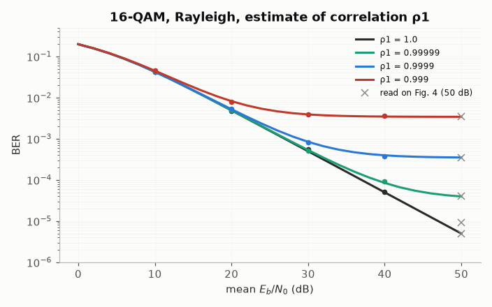
• M.-X. Chang and Y. T. Su, “Performance analysis of equalized OFDM systems in Rayleigh fading,” IEEE Trans. Wireless Commun. 1(4), 721–732, 2002: the bit error rate of a receiver that equalises with a pilot-assisted channel estimate (comnum.theory_ber_imperfect_csi(), comnum.theory_ber_dpsk_jakes());

• P. Banelli and S. Cacopardi, “Theoretical analysis and performance of OFDM signals in nonlinear AWGN channels,” IEEE Trans. Commun. 48(3), 430–441, 2000: the distortion of an amplifier driven by an OFDM signal and the resulting bit error rate (comnum.envelope_series(), comnum.distortion_spectrum()).

Sources and how they are used. The formulas are those of the papers, with their equation numbers; the comparison values marked “read on the figure” were read by eye on the PDF figures, to about 10 % — they check the order of magnitude and the trends, not the digits. The tests are validation/tests/synchronisation/chang2002.rs and validation/tests/hardware/banelli2000.rs. Reproducing the papers found four misprints, each settled by an exact computation or by the paper’s own figures:

• Chang & Su, Sec. IV-D3: the asymptote of 16-QAM is \(0.4972/\bar\gamma_b\) (the expansion of their eq. 69), printed \(0.4952/\bar\gamma_b\);

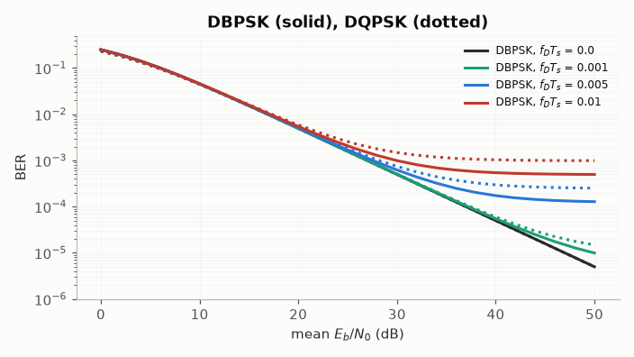
• Chang & Su, Fig. 3: the curve labelled \(f_D T_s = 0.05\) floors where their eq. 40 puts \(f_D T_s = 0.005\);

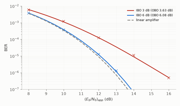
• Banelli & Cacopardi, eq. 31: the output back-off is \(\gamma/(1 - e^{-\gamma})\) (it gives the 3.64 and 6.08 dB of their Fig. 5), printed \(\gamma \cdot (1 - e^{-\gamma})\);

• Banelli & Cacopardi, eq. 28 and Table I: the exact integral of their eq. 7 needs \(+\sum_i d_{i,n}\gamma^{i+1}\) with the coefficients of Table I, printed with a minus sign; the magnitudes of the table are exact.

import matplotlib.pyplot as plt
import numpy as np

import comnum
from comnum.plot import BLUE, CRIMSON, GREY, LABEL, TEAL

rng = comnum.Rng(32)

Imperfect channel estimates (Chang & Su)

Every linear pilot-assisted estimate \(\hat H\) (least squares, LMMSE, interpolation) is jointly Gaussian with the channel \(H\); the bit error rate then depends on their correlation \(\rho_1 + j\rho_2\) only (their eqs. 31, 32, 53). A correlation of 0.999 — an estimate 30 dB better than the channel — still leaves 16-QAM with an error floor near \(3.4 \cdot 10^{-3}\) (their Fig. 4). The markers are a Monte Carlo simulation of that model with the 16-QAM of comnum.

c16 = comnum.Constellation("qam", 16).normalized()


def simulate_16qam(ebn0_db, rho, n=150_000):
    idx = rng.integers(16, n)
    h = rng.complex_noise(n, 1.0)
    hh = rho * h + rng.complex_noise(n, 1.0 - rho**2)
    n0 = 1 / (4 * comnum.db2lin(ebn0_db))
    y = h * c16.points[idx] + rng.complex_noise(n, n0)
    dec = c16.demap_bits(y / hh)
    return np.mean(dec != comnum.unpack_symbols(idx.astype(np.uint16), 4)[: 4 * n])


ebn0 = np.arange(0.0, 51.0, 2.0)
fig, ax = plt.subplots(figsize=(6.4, 4.0))
for rho, color in [(1.0, LABEL), (0.99999, TEAL), (0.9999, BLUE), (0.999, CRIMSON)]:
    ax.semilogy(
        ebn0, comnum.theory_ber_imperfect_csi("16qam", ebn0, rho), color=color, label=f"ρ1 = {rho}"
    )
    pts = np.arange(10.0, 41.0, 10.0)
    ax.semilogy(pts, [simulate_16qam(e, rho) for e in pts], "o", color=color, markersize=4)
read = {1.0: 5e-6, 0.999999: 9e-6, 0.99999: 4e-5, 0.9999: 3.5e-4, 0.999: 3.5e-3}
ax.semilogy([50] * len(read), list(read.values()), "x", color=GREY, label="read on Fig. 4 (50 dB)")
ax.set(
    xlabel="mean $E_b/N_0$ (dB)",
    ylabel="BER",
    ylim=(1e-6, 0.5),
    title="16-QAM, Rayleigh, estimate of correlation ρ1",
)
ax.grid(alpha=0.3, which="both")
ax.legend(fontsize=8)
fig.tight_layout()

Differential detection over Jakes’ fading

Without an estimate, DPSK compares two symbols; the channel decorrelates between them as \(J_0(2\pi f_D T_s)\) and the error rate floors at \(\frac{1}{2}(1 - J_0(2\pi f_D T_s))\) for DBPSK (their eq. 40).

fig, ax = plt.subplots(figsize=(6.4, 3.6))
for fd, color in [(0.0, LABEL), (0.001, TEAL), (0.005, BLUE), (0.01, CRIMSON)]:
    ax.semilogy(
        ebn0,
        comnum.theory_ber_dpsk_jakes(2, ebn0, fd),
        color=color,
        label=f"DBPSK, $f_D T_s$ = {fd}",
    )
    ax.semilogy(ebn0, comnum.theory_ber_dpsk_jakes(4, ebn0, fd), ":", color=color)
ax.set(
    xlabel="mean $E_b/N_0$ (dB)",
    ylabel="BER",
    ylim=(1e-6, 0.5),
    title="DBPSK (solid), DQPSK (dotted)",
)
ax.grid(alpha=0.3, which="both")
ax.legend(fontsize=8)
fig.tight_layout()

A nonlinear amplifier driven by OFDM (Banelli & Cacopardi)

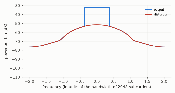
An ideally predistorted amplifier clips the envelope at \(A\); the input back-off is \(\gamma = A^2/P_{\mathrm{in}}\). The output autocorrelation is a series whose term \(n\) has the input spectrum convolved \(2n + 1\) times with itself: the distortion spreads outside the band and is not white inside it. Here the DAB signal of their Fig. 5: 1536 subcarriers of 2048, oversampled four times, at 3 dB of input back-off.

gamma = comnum.db2lin(3)
c = comnum.envelope_series(lambda r: np.minimum(r, np.sqrt(gamma)), 60)
bins, occupied = 8192, 1536
useful, dist = comnum.distortion_spectrum(c, occupied, bins)
f = np.fft.fftshift(np.fft.fftfreq(bins, 1 / 4.0))
fig, ax = plt.subplots(figsize=(6.4, 3.4))
ax.plot(f, comnum.lin2db(np.fft.fftshift(useful + dist) + 1e-30), color=BLUE, label="output")
ax.plot(f, comnum.lin2db(np.fft.fftshift(dist) + 1e-30), color=CRIMSON, label="distortion")
ax.set(
    xlabel="frequency (in units of the bandwidth of 2048 subcarriers)",
    ylabel="power per bin (dB)",
    ylim=(-110, -30),
)
ax.grid(alpha=0.3)
ax.legend(fontsize=8)
fig.tight_layout()

Bit error rate of DQPSK through the amplifier

On every subcarrier the distortion adds to the noise as a Gaussian term (their eqs. 17–21); the curves average the BER of DQPSK over the subcarriers, against the apparent \(E_b/N_0\) (the noise alone). The crosses are the points read on their Fig. 5 for input back-offs of 3 and 6 dB (output back-offs 3.64 and 6.08 dB in the paper; 3.63 dB here for exactly 3 dB, the paper’s 3.64 dB being \(\gamma = 2\)).

carriers = (np.arange(occupied) - occupied // 2) % bins
x_app = np.arange(8.0, 16.1, 0.5)
fig, ax = plt.subplots(figsize=(6.4, 3.8))
for ibo, color, pts in [
    (3.0, CRIMSON, [(8, 6e-3), (10, 1.2e-3), (12, 1.25e-4), (14, 1.1e-5), (16, 5e-7)]),
    (6.0, BLUE, [(8, 3.7e-3), (10, 3.7e-4), (12, 1.3e-5), (13, 1.3e-6)]),
]:
    g = comnum.db2lin(ibo)
    a = np.sqrt(g)
    cc = comnum.envelope_series(lambda r, a=a: np.minimum(r, a), 60)
    u, d = comnum.distortion_spectrum(cc, occupied, bins)
    sdr = u[carriers] / d[carriers]
    ber = [
        np.mean(
            comnum.theory_ber_dpsk(4, comnum.lin2db(1 / (1 / sdr + 1 / (2 * comnum.db2lin(x))) / 2))
        )
        for x in x_app
    ]
    obo = comnum.lin2db(g / (1 - np.exp(-g)))
    ax.semilogy(x_app, ber, color=color, label=f"IBO {ibo:.0f} dB (OBO {obo:.2f} dB)")
    ax.semilogy(*zip(*pts, strict=True), "x", color=color, markersize=7)
ax.semilogy(x_app, comnum.theory_ber_dpsk(4, x_app), "--", color=GREY, label="linear amplifier")
ax.set(xlabel="$(E_b/N_0)_{app}$ (dB)", ylabel="BER", ylim=(1e-7, 1e-2))
ax.grid(alpha=0.3, which="both")
ax.legend(fontsize=8)
fig.tight_layout()