OFDM over multipath: channel estimation

A multipath channel is frequency selective, but OFDM with a cyclic prefix longer than its delay spread sees it as one flat fading coefficient per subcarrier, which a one-tap equaliser removes — provided the receiver knows it. The channel here is the Extended Vehicular A profile of 3GPP TS 36.101 (nine taps, 357 ns RMS delay spread) at a sampling rate of 3.84 MHz, with Clarke/Jakes Doppler (Zheng & Xiao 2003).

Pilots on a lattice (one subcarrier in 3, one symbol in 4; Coleri et al. 2002) give least-squares estimates, interpolated across the subcarriers — linearly, or by linear MMSE with the frequency correlation of the channel (van de Beek et al. 1995), the true one or the uniform profile over the cyclic prefix of the robust design (Edfors et al. 1998) — and linearly in time.

import matplotlib.pyplot as plt
import numpy as np

import comnum
from comnum.plot import BACKGROUND, GREY

N, K, CP, FS = 256, 200, 16, 3.84e6
ofdm = comnum.Ofdm(N, K, oversampling=1, n_cp=CP)
c = comnum.Constellation("qam", 4).normalized()

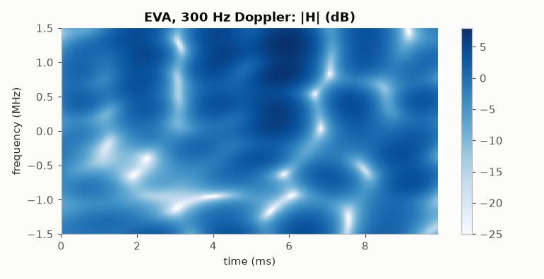
The channel seen by the grid: the magnitude of H(k, l) for an EVA realisation at a Doppler of 300 Hz over 140 OFDM symbols (about 10 ms).

L = 140
ch = comnum.TdlChannel("eva", FS, doppler_hz=300.0)
x = ofdm.modulate(np.ones(K * L))
_, taps = ch.fade(x, comnum.Rng(1))
H = np.stack(
    [
        np.abs(taps.frequency_response(sym * ofdm.block_len, ofdm.bins, N)[:, 0, 0])
        for sym in range(L)
    ]
)
fig, ax = plt.subplots(figsize=(7.0, 3.6))
im = ax.imshow(
    20 * np.log10(H.T),
    aspect="auto",
    origin="lower",
    cmap="Blues",
    vmin=-25,
    vmax=8,
    extent=(0, L * ofdm.block_len / FS * 1e3, -K / 2 * FS / N / 1e6, K / 2 * FS / N / 1e6),
)
ax.set(xlabel="time (ms)", ylabel="frequency (MHz)", title="EVA, 300 Hz Doppler: |H| (dB)")
ax.grid(False)
fig.colorbar(im, ax=ax)
fig.tight_layout()

Estimation error and bit error rate over static EVA realisations (one per grid of 14 symbols), QPSK.

def link(eb, estimator, frames=150, seed=1):
    grid = comnum.ResourceGrid(K, 14, pattern="lattice", freq=3, time=4, seed=1)
    ch = comnum.TdlChannel("eva", FS)
    err = tot = 0
    mse = 0.0
    for f in range(frames):
        rng = comnum.Rng.stream(seed, "ofdm", int(eb * 10), f)
        bits = comnum.bits(2 * grid.n_data, rng)
        x = ofdm.modulate(grid.map(c.map_bits(bits)))
        y, taps = ch.fade(x, rng)
        s2 = N / (2 * K * comnum.db2lin(eb))
        rx = ofdm.demodulate(y + rng.complex_noise(y.size, s2))
        h = np.tile(taps.frequency_response(0, ofdm.bins, N)[:, 0, 0], 14)
        nv = s2 * K / N
        if estimator == "perfect CSI":
            hh = h
        elif estimator == "LMMSE, true profile":
            hh = comnum.ofdm_estimate(
                grid,
                rx,
                nv,
                "lmmse",
                delays=[float(d) for d in taps.delays],
                powers=ch.powers,
                n_fft=N,
            )
        elif estimator == "LMMSE, robust":
            hh = comnum.ofdm_estimate(grid, rx, nv, "lmmse", max_delay=CP, n_fft=N)
        else:
            hh = comnum.ofdm_estimate(grid, rx, nv, "linear")
        mse += np.mean(np.abs(hh - h) ** 2) / frames
        err += int((c.demap_bits(grid.extract(rx / hh)) != bits).sum())
        tot += bits.size
    return err / tot, mse


ebs = np.arange(0.0, 31.0, 5.0)
names = ["linear interpolation", "LMMSE, robust", "LMMSE, true profile", "perfect CSI"]
res = {n: [link(e, n) for e in ebs] for n in names}
fig, (ax1, ax2) = plt.subplots(1, 2, figsize=(9.5, 3.9))
for name, marker in zip(names[:3], ["o", "s", "D"], strict=True):
    ax1.semilogy(
        ebs, [r[1] for r in res[name]], marker=marker, markeredgecolor=BACKGROUND, label=name
    )
ax1.set(xlabel="$E_b/N_0$ (dB)", ylabel="MSE of the channel estimate", title="estimation error")
ax1.legend()
fine = np.linspace(0, 30, 121)
ax2.semilogy(
    fine,
    comnum.theory_ber_rayleigh_mrc(fine, branches=1),
    color=GREY,
    linewidth=1.4,
    label="Rayleigh, theory",
)
for name, marker in zip(names, ["o", "s", "D", "^"], strict=True):
    ax2.semilogy(
        ebs, [r[0] for r in res[name]], marker=marker, markeredgecolor=BACKGROUND, label=name
    )
ax2.set(
    xlabel="$E_b/N_0$ (dB)", ylabel="bit error rate", title="QPSK OFDM over EVA", ylim=(1e-4, 0.3)
)
ax2.legend(fontsize=8)
fig.tight_layout()

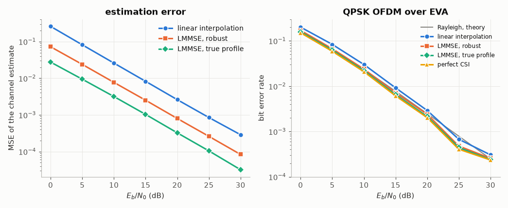
With perfect CSI every subcarrier is a flat Rayleigh channel: the BER is that of BPSK over Rayleigh fading with coherent detection, 0.5 (1 - sqrt(γ/(1 + γ))).

eb = 10.0
print(
    f"{eb} dB: simulated {res['perfect CSI'][2][0]:.4f}, theory "
    f"{comnum.theory_ber_rayleigh_mrc(eb, branches=1):.4f}"
)

10.0 dB: simulated 0.0209, theory 0.0233