Nyquist pulse shaping and the eye diagram

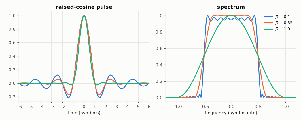
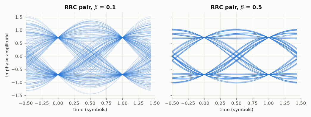
A root-raised-cosine (RRC) transmit filter followed by the same matched filter at the receiver gives a raised-cosine overall response, whose zero crossings at every other symbol instant cancel the intersymbol interference (Nyquist’s criterion). The roll-off \(\beta\) trades bandwidth, \((1 + \beta) R_s\), against the length of the pulse tails and the sensitivity to timing errors — which the eye diagram shows.

import matplotlib.pyplot as plt
import numpy as np

import comnum
from comnum.plot import BLUE

SPS = 16
fig, (ax1, ax2) = plt.subplots(1, 2, figsize=(9.5, 3.8))
for beta in [0.1, 0.35, 1.0]:
    h = comnum.pulse_shape("rc", SPS, n_taps=16 * SPS + 1, rolloff=beta)
    t = (np.arange(h.size) - h.size // 2) / SPS
    ax1.plot(t, h / h.max(), label=rf"$\beta$ = {beta}")
    H = np.abs(np.fft.fftshift(np.fft.fft(h, 4096)))
    f = np.fft.fftshift(np.fft.fftfreq(4096, 1 / SPS))
    ax2.plot(f, H / H.max(), label=rf"$\beta$ = {beta}")
ax1.set(xlim=(-6, 6), xlabel="time (symbols)", title="raised-cosine pulse")
ax1.set_xticks(range(-6, 7))
ax2.set(xlim=(-1.2, 1.2), xlabel="frequency (symbol rate)", title="spectrum")
ax2.legend()
fig.tight_layout()

Eye diagrams of QPSK (in phase) after the RRC pair: wide open with a large roll-off, narrower — and closing quickly with a timing error — with a small one.

c = comnum.Constellation("qam", 4).normalized()
_, x = comnum.symbols(c, 600, comnum.Rng(3))
fig, axes = plt.subplots(1, 2, figsize=(9.5, 3.6), sharey=True)
for ax, beta in zip(axes, [0.1, 0.5], strict=True):
    h = comnum.pulse_shape("rrc", SPS, n_taps=32 * SPS + 1, rolloff=beta)
    y = comnum.fir_filter(h, comnum.fir_filter(h, comnum.upsample(x, SPS)))
    y = y / np.sqrt(np.mean(np.abs(y[::SPS]) ** 2))
    # two-symbol windows centred on the sampling instants t = 0 and t = 1
    traces = y[40 * SPS - SPS // 2 : 560 * SPS - SPS // 2].real.reshape(-1, 2 * SPS)
    t = np.arange(2 * SPS) / SPS - 0.5
    ax.plot(t, traces.T, color=BLUE, linewidth=0.6, alpha=0.25)
    ax.set(title=rf"RRC pair, $\beta$ = {beta}", xlabel="time (symbols)", xlim=(-0.5, 1.5))
axes[0].set_ylabel("in-phase amplitude")
fig.tight_layout()