Looking at the signals along a chain

Three ways to see what a block does to the signal. comnum.Chain.trace() runs one trial and keeps the frame after every block, for plots and NumPy; probe blocks measure metrics at a point of the link during a whole campaign; the dump block saves the samples at a point of the link for the first trials of every condition, as SigMF recordings that any tool reads. A Python block can also keep whatever it wants. The chain is the coherent receiver of specs/coherent_link.yaml.

import tempfile
from pathlib import Path

import matplotlib.pyplot as plt
import numpy as np
from _gallery_utils import SPECS

import comnum
from comnum import blocks as B

spec = SPECS / "coherent_link.yaml"
link = comnum.Chain.from_spec(spec)
condition = {"length_km": 1000, "snr_db": 18}

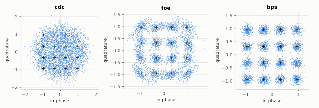
Trace. The frame after every block of one trial: its samples, samples per symbol, and what the source recorded (bits, symbols, constellation). Trace.plot draws one panel per stage with a function of comnum.plot; the functions take a frame directly and read its sampling rate and constellation.

frames = link.trace(condition, comnum.Rng(1))
for name, f in frames.items():
    print(f"{name:>16}: {f.samples.size:>6} samples at {f.sps:g} per symbol")
fig = frames.plot("constellation", stages=["cdc", "foe", "bps"], skip=2560, max_points=4000)
fig.set_size_inches(10, 3.4)
fig.tight_layout()

        source:  16384 samples at 1 per symbol
   pulse_shape:  32768 samples at 2 per symbol
      tx_laser:  32768 samples at 2 per symbol
         fiber:  32768 samples at 2 per symbol
     normalize:  32768 samples at 2 per symbol
          awgn:  32768 samples at 2 per symbol
      lo_laser:  32768 samples at 2 per symbol
           cfo:  32768 samples at 2 per symbol
           cdc:  32768 samples at 2 per symbol
matched_filter:  32768 samples at 2 per symbol
       gardner:  32750 samples at 2 per symbol
      decimate:  16375 samples at 1 per symbol
           foe:  16375 samples at 1 per symbol
           bps:  16375 samples at 1 per symbol
    frame_sync:  16384 samples at 1 per symbol

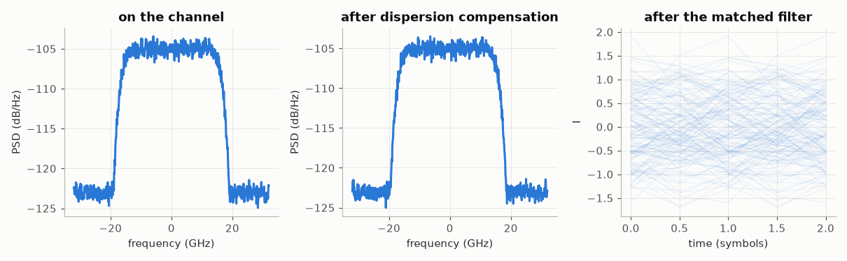
The spectrum before and after dispersion compensation, and the eye after the matched filter.

fig, axes = plt.subplots(1, 3, figsize=(11, 3.4))
comnum.plot.psd(frames["awgn"], ax=axes[0])
axes[0].set_title("on the channel")
comnum.plot.psd(frames["cdc"], ax=axes[1])
axes[1].set_title("after dispersion compensation")
comnum.plot.eye(frames["matched_filter"], ax=axes[2], traces=150, skip=4096)
axes[2].set_title("after the matched filter")
fig.tight_layout()

Probes. During a campaign, a probe after a block measures metrics there, on every trial, reported as <block>.<metric> with their intervals. The power and the PAPR are measured anywhere; the metrics on decisions (SNR, EVM, error rates) need the samples aligned on the transmitted symbols, here after frame synchronisation.

probed = link.probes(
    {"awgn": ["power_dbm", "papr_db"], "cdc": ["papr_db"], "frame_sync": ["snr_db", "evm"]},
    skip_start=2560,
    skip_end=256,
)
res = probed.run(
    grid={"length_km": [1000], "snr_db": [14, 18]}, metrics=["ber"], stop={"max_trials": 8}
)
for r in res:
    m = r["metrics"]
    print(
        f"SNR {r['condition']['snr_db']} dB: {m['awgn.power_dbm']['value']:.1f} dBm on the channel, "
        f"PAPR {m['awgn.papr_db']['value']:.1f} dB on the channel and {m['cdc.papr_db']['value']:.1f} dB "
        f"after dispersion compensation; {m['frame_sync.snr_db']['value']:.1f} dB and "
        f"EVM {100 * np.sqrt(m['frame_sync.evm']['value']):.1f} % at the decisions"
    )

SNR 14 dB: 30.3 dBm on the channel, PAPR 10.5 dB on the channel and 7.4 dB after dispersion compensation; 13.8 dB and EVM 20.5 % at the decisions
SNR 18 dB: 30.1 dBm on the channel, PAPR 10.3 dB on the channel and 6.9 dB after dispersion compensation; 17.3 dB and EVM 13.6 % at the decisions

Dumps. A dump block saves the samples at its position for the first trials of every condition (trials of them), as SigMF recordings <dir>/<campaign>/<condition>/<label>_<trial>.sigmf-* with the samples per symbol and the symbol rate in their metadata; the campaign goes on as usual on every core. comnum.read_sigmf() reads them back, as does any SigMF tool.

folder = Path(tempfile.mkdtemp())
tapped = link.insert_after("cdc", tap=B.Dump(dir=str(folder), trials=1))
tapped.run(
    grid={"length_km": [1000], "snr_db": [14, 18]},
    metrics=["ber"],
    stop={"max_trials": 4},
    name="taps",
)
for p in sorted(folder.rglob("*.sigmf-meta")):
    print(p.relative_to(folder))
x, fs, meta = comnum.read_sigmf(folder / "taps" / "length_km=1000_snr_db=18" / "tap_0.sigmf-meta")
print(
    x.shape,
    f"{fs / 1e9:.0f} GHz,",
    {k: v for k, v in meta["global"].items() if k.startswith("comnum:")},
)

taps/length_km=1000_snr_db=14/tap_0.sigmf-meta
taps/length_km=1000_snr_db=18/tap_0.sigmf-meta
(32768,) 64 GHz, {'comnum:block': 'tap', 'comnum:trial': 0, 'comnum:stream': 0, 'comnum:sps': 2.0, 'comnum:symbol_rate': 32000000000.0}

The first trial of a condition draws from Rng.stream(seed, name, i, 0), so the recording is exactly the frame that trace gives with that generator: a dump of the parallel runner and a trace in Python are the same signal.

i = 1  # the condition snr_db = 18 is the second of the grid
same = tapped.trace({"length_km": 1000, "snr_db": 18}, comnum.Rng.stream(7, "taps", i, 0))
print("dump and trace agree:", np.array_equal(same["cdc"].samples, x))

dump and trace agree: True

A Python block as a tap. On the Python runner, a block is any callable: one that appends a copy of the samples to a list keeps every trial of the campaign in memory, which a dump would write to disk.

kept = []


def keep(frame, rng):
    kept.append(frame.samples.copy())


link.insert_after("bps", keep=keep).run(
    grid={"length_km": [1000], "snr_db": [18]}, metrics=["ber"], stop={"max_trials": 8}
)
print(len(kept), "trials kept,", kept[0].shape)

8 trials kept, (16375,)

Saving a trace. Trace.save writes the samples of every stage to a .npz file, under stage/<name>/ for every block, for NumPy or any tool that reads them.

path = frames.save(folder / "trace.npz")
with np.load(path) as z:
    print(sorted(z.files)[:6], "…")

['stage/awgn/sps', 'stage/awgn/stream0', 'stage/bps/sps', 'stage/bps/stream0', 'stage/cdc/sps', 'stage/cdc/stream0'] …