A first link: 16-QAM over AWGN

The smallest complete simulation: draw bits, map them on a constellation, add noise, decide, count the errors and compare with the closed form. Every step is one call on NumPy arrays. The same link is then written as a chain of named blocks and run as a Monte Carlo campaign on every core, with a stopping rule and confidence intervals.

import matplotlib.pyplot as plt
import numpy as np

import comnum
from comnum import blocks as B
from comnum.plot import BACKGROUND, MUTED

The generator. There is no global random state: every function that draws takes a comnum.Rng and advances it, so a script is reproducible from its seed (and gives the same numbers as the Rust crates).

rng = comnum.Rng(2024)

The constellation. Constellation(kind, m) carries the points and their Gray labels; normalized() scales them to a unit average energy, the convention of the closed forms. demodulate on the points themselves returns the label of each.

c = comnum.Constellation("qam", 16).normalized()
k = c.bits_per_symbol
labels = c.demap_bits(c.points).reshape(-1, k)
print(c, "-", k, "bits per symbol, energy", np.mean(np.abs(c.points) ** 2))

fig, ax = plt.subplots(figsize=(4.4, 4.4))
ax.plot(c.points.real, c.points.imag, "o", markersize=7)
for p, bits in zip(c.points, labels, strict=True):
    ax.annotate("".join(map(str, bits)), (p.real, p.imag), (6, 6), textcoords="offset points",
                fontsize=8, color=MUTED)  # fmt: skip
ax.set(aspect="equal", xlabel="in phase", ylabel="quadrature", title="16-QAM, Gray labels")
fig.tight_layout()

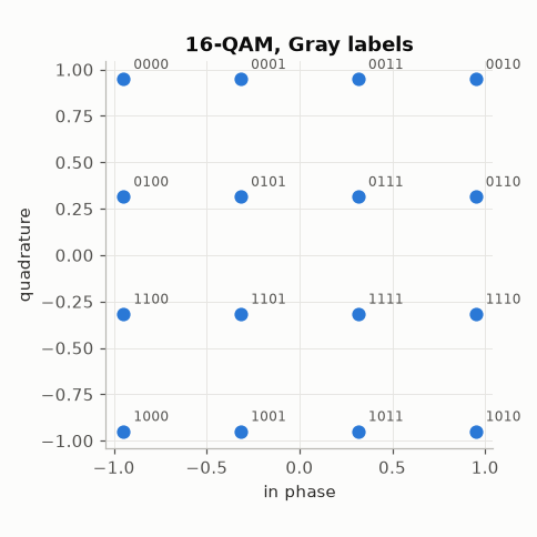
comnum.Constellation('qam', 16, energy=1.000000) - 4 bits per symbol, energy 1.0
findfont: Failed to find font weight semibold for DejaVu Sans, now using 700.

Bits, symbols, noise, decisions. comnum.awgn_ebn0() adds the noise for an \(E_b/N_0\) in dB, given the bits per symbol; demodulate decides the nearest point and returns its bits; comnum.ber() counts the differences.

bits = comnum.bits(k * 100_000, rng)
x = c.map_bits(bits)
y = comnum.awgn_ebn0(x, 10.0, k, rng)
decided = c.demap_bits(y)
print(f"BER {comnum.ber(decided, bits):.2e}, closed form {comnum.theory_ber(16, 10.0, 'qam'):.2e}")

fig, ax = plt.subplots(figsize=(4.4, 4.4))
comnum.plot.constellation(y, ax=ax, reference=c, max_points=8000)
ax.set_title("received at $E_b/N_0$ = 10 dB")
fig.tight_layout()

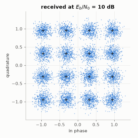
BER 1.76e-03, closed form 1.75e-03
findfont: Failed to find font weight semibold for DejaVu Sans, now using 700.

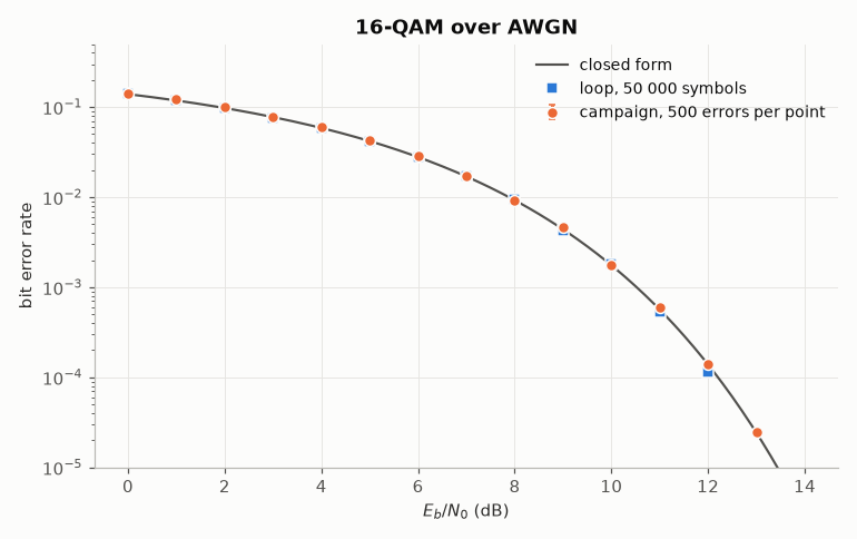
A sweep by hand. A loop over \(E_b/N_0\) gives a first curve. What sets the precision of a point is its number of errors: with 100 errors the relative standard error is about 10 %, with 400 about 5 %. The points of the loop below are left out once they have fewer than 20 errors.

ebn0 = np.arange(0.0, 15.0, 1.0)
ber_loop = []
for e in ebn0:
    bits = comnum.bits(k * 50_000, rng)
    y = comnum.awgn_ebn0(c.map_bits(bits), e, k, rng)
    errors = int((c.demap_bits(y) != bits).sum())
    ber_loop.append(errors / bits.size if errors >= 20 else np.nan)

The same link as a chain. A comnum.Chain names the blocks of the link; comnum.var() marks the parameter that the campaign sweeps. run evaluates the chain on a grid of conditions on the parallel Rust runner, until a stopping rule is met (here 500 bit errors, or 2000 trials of 4096 symbols), and reports every metric with its 95 % confidence interval.

link = comnum.Chain(
    tx=B.Source(constellation="16-QAM", n_symbols=4096),
    channel=B.AwgnEbn0(ebn0_db=comnum.var("ebn0_db")),
)
results = link.run(
    grid={"ebn0_db": list(ebn0)},
    metrics=["ber", "ser"],
    stop={"min_errors": {"ber": 500}, "max_trials": 2000},
    seed=1,
)
r = results.where(ebn0_db=10.0)[0]
print(r["condition"], r["trials"], "trials,", r["metrics"]["ber"])

{'ebn0_db': 10.0} 32 trials, {'value': 0.0017566680908203125, 'lo': 0.0016469091183436224, 'hi': 0.0018737282688121937, 'kind': 'rate', 'count': 921, 'total': 524288}

The loop, the campaign with its intervals, and the closed form of Gray-mapped QAM (Proakis & Salehi, Digital Communications, 5th ed., Sec. 4.3-2).

x, ber, lo, hi = results.series("ebn0_db", "ber", interval=True)
fine = np.linspace(0, 14, 141)
fig, ax = plt.subplots()
ax.semilogy(fine, comnum.theory_ber(16, fine, "qam"), color=MUTED, linewidth=1.4,
            label="closed form")  # fmt: skip
ax.semilogy(ebn0, ber_loop, "s", markeredgecolor=BACKGROUND, label="loop, 50 000 symbols")
ax.errorbar(x, ber, yerr=[ber - lo, hi - ber], fmt="o", markeredgecolor=BACKGROUND, capsize=2,
            label="campaign, 500 errors per point")  # fmt: skip
ax.set(ylim=(1e-5, 0.5), xlabel="$E_b/N_0$ (dB)", ylabel="bit error rate", title="16-QAM over AWGN")
ax.legend()
fig.tight_layout()

Where to go next. A classical single-carrier chain adds pulse shaping, a matched filter and impairments to this link; the user guide describes chains, probes and variants; Specifications and the command line runs the same campaign from a YAML file and the command line.