A classical single-carrier chain

QPSK at several samples per symbol: root-raised-cosine pulse shaping, additive noise, the matched filter and decimation to one sample per symbol — the textbook chain, as a comnum.Chain of native blocks. The chain runs once to look at the signals after every block (the eye diagram, the spectrum, the constellation), then as a campaign against the closed form; variants with laser phase noise and blind phase search are one line apart.

import matplotlib.pyplot as plt
import numpy as np

import comnum
from comnum import blocks as B

The chain. The blocks are the classes of comnum.blocks, one per entry of comnum.spec_blocks(); help(B.PulseShape) lists the parameters of a block with their defaults and units. Awgn sets the SNR per symbol: its noise bandwidth is the symbol rate by default, whatever the samples per symbol.

SPS, ROLLOFF = 8, 0.35
link = comnum.Chain(
    tx=B.Source(constellation="QPSK", n_symbols=4096),
    shaping=B.PulseShape(kind="rrc", sps=SPS, rolloff=ROLLOFF, n_taps=129),
    channel=B.Awgn(snr_db=comnum.var("snr_db")),
    mf=B.MatchedFilter(kind="rrc", rolloff=ROLLOFF, n_taps=129),
    down=B.Decimate(),
)
print(link)

Chain(
    tx=Source(constellation='QPSK'),
    shaping=PulseShape(rolloff=0.35, n_taps=129, sps=8),
    channel=Awgn(snr_db=var('snr_db')),
    mf=MatchedFilter(rolloff=0.35, n_taps=129),
    down=Decimate()
)

One run, traced. trace runs the chain once and keeps a copy of the frame after every block. A frame carries the samples, the samples per symbol and what the metrics need (the transmitted bits and symbols, the constellation).

frames = link.trace({"snr_db": 15.0}, comnum.Rng(1))
for name, f in frames.items():
    print(f"{name:>8}: {f.samples.size} samples, {f.sps:g} per symbol")

     tx: 4096 samples, 1 per symbol
shaping: 32768 samples, 8 per symbol
channel: 32768 samples, 8 per symbol
     mf: 32768 samples, 8 per symbol
   down: 4096 samples, 1 per symbol

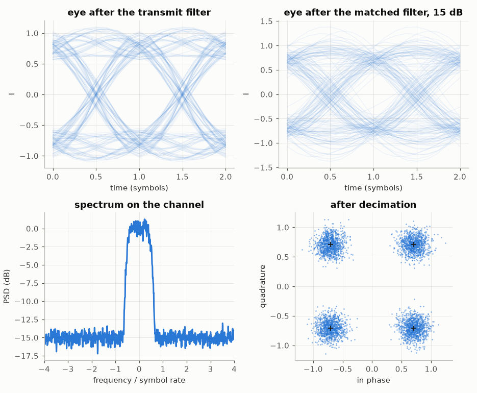
The eye diagram after shaping is open at the sampling instants only after the matched filter (a root-raised cosine alone is not a Nyquist pulse); the spectrum has the roll-off of the pulse; the samples before and after decimation.

fig, axes = plt.subplots(2, 2, figsize=(8.5, 7))
comnum.plot.eye(frames["shaping"], ax=axes[0, 0], traces=200)
axes[0, 0].set_title("eye after the transmit filter")
comnum.plot.eye(frames["mf"], ax=axes[0, 1], traces=200)
axes[0, 1].set_title("eye after the matched filter, 15 dB")
comnum.plot.psd(frames["channel"], ax=axes[1, 0])
axes[1, 0].set(title="spectrum on the channel", xlim=(-SPS / 2, SPS / 2))
comnum.plot.constellation(frames["down"], ax=axes[1, 1])
axes[1, 1].set_title("after decimation")
fig.tight_layout()

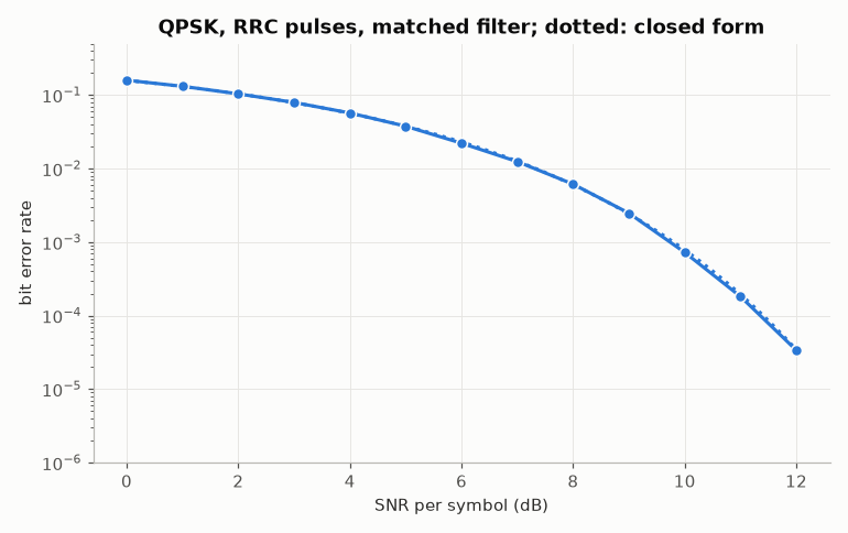
The campaign. skip_start and skip_end leave the transients of the filters out of the metrics. The SNR per symbol of Awgn is \(E_s/N_0\), so the closed form of QPSK is that of 4-QAM at \(E_b/N_0 = E_s/N_0 - 3\,\mathrm{dB}\).

campaign = {
    "grid": {"snr_db": list(np.arange(0.0, 13.0, 1.0))},
    "metrics": {"report": ["ber"], "skip_start": 64, "skip_end": 64},
    "stop": {"min_errors": {"ber": 400}, "max_trials": 1000},
    "seed": 1,
}
results = link.run(**campaign)


def qpsk(snr_db):
    return comnum.theory_ber(4, np.asarray(snr_db) - comnum.lin2db(2), "qam")


fig, ax = plt.subplots()
results.plot("snr_db", "ber", ax=ax, theory=qpsk)
ax.set(xlabel="SNR per symbol (dB)", ylabel="bit error rate", ylim=(1e-6, 0.5),
       title="QPSK, RRC pulses, matched filter; dotted: closed form")  # fmt: skip
fig.tight_layout()

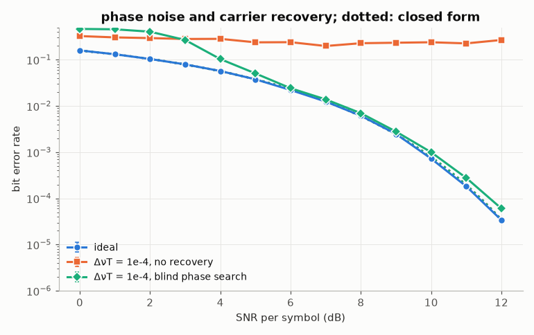
Variants. insert_after and replace return modified copies of the chain. A laser of linewidth \(\Delta\nu\) adds a Wiener phase noise of variance \(2\pi\Delta\nu T\) per symbol (\(T\) is the symbol period; the time axis of the source is normalised, so linewidth_hz is \(\Delta\nu T\)). Blind phase search (Pfau, Hoffmann & Noé 2009) estimates the phase from the decisions over a sliding window of \(2n + 1\) symbols, and FrameSync resolves the four-fold ambiguity of QPSK on the known symbols. Without recovery the phase walks away within a few hundred symbols; with it the loss is a fraction of a dB. comnum.compare() runs the variants with the same grid and gathers them.

noisy = link.insert_after("channel", laser=B.PhaseNoise(linewidth_hz=1e-4))
recovered = noisy.insert_after("down", cpr=B.Bps(n=32, b=32), sync=B.FrameSync())
variants = {
    "ideal": link,
    "ΔνT = 1e-4, no recovery": noisy,
    "ΔνT = 1e-4, blind phase search": recovered,
}
res = comnum.compare(variants, **campaign)

fig, ax = plt.subplots()
res.plot("snr_db", "ber", by="variant", ax=ax, theory=lambda s, _: qpsk(s))
ax.set(xlabel="SNR per symbol (dB)", ylabel="bit error rate", ylim=(1e-6, 0.5),
       title="phase noise and carrier recovery; dotted: closed form")  # fmt: skip
fig.tight_layout()

Probes. probe measures metrics at a point of the chain during the whole campaign, reported as <block>.<metric>: here the power of the shaped signal and the SNR estimated from the decisions after carrier recovery, which the phase noise lowers by a fraction of a dB.

probed = recovered.probes(
    {"shaping": ["power_dbm"], "sync": ["snr_db"]}, skip_start=64, skip_end=64
)
res = probed.run(grid={"snr_db": [6.0, 10.0, 14.0]}, metrics=["ber"], stop={"max_trials": 16})
for r in res:
    m = r["metrics"]
    print(
        f"SNR {r['condition']['snr_db']:>4} dB: {m['shaping.power_dbm']['value']:.1f} dBm "
        f"after shaping, {m['sync.snr_db']['value']:.1f} dB estimated after carrier recovery"
    )

SNR  6.0 dB: 30.0 dBm after shaping, 6.7 dB estimated after carrier recovery
SNR 10.0 dB: 30.0 dBm after shaping, 10.2 dB estimated after carrier recovery
SNR 14.0 dB: 30.0 dBm after shaping, 13.8 dB estimated after carrier recovery