Where the time goes: profiling a chain

A campaign run with profile=True times every block of every trial and reports the mean time per trial of each as a metric, <block>.time_ms, next to the error rates. comnum.Results.profile() turns these metrics into a table, in the order of the link, with the share of every block; comnum.Chain.profile() runs a short campaign and returns it. The same table comes from the command line with comnum run --profile. This tutorial profiles the coherent receiver of specs/coherent_link.yaml, compares two settings of its carrier recovery, and measures the price of a block written in Python.

import matplotlib.pyplot as plt
import numpy as np
from _gallery_utils import SPECS

import comnum
from comnum import blocks as B

spec = SPECS / "coherent_link.yaml"
link = comnum.Chain.from_spec(spec)
print(link.names)

['source', 'pulse_shape', 'tx_laser', 'fiber', 'normalize', 'awgn', 'lo_laser', 'cfo', 'cdc', 'matched_filter', 'gardner', 'decimate', 'foe', 'bps', 'frame_sync']

The profile of one condition. Sixteen trials of 16 384 symbols at 1000 km. The times are wall-clock times of one trial on one core; the parallel runner runs as many trials at once as there are cores, so the throughput of a campaign is about the number of cores divided by link.time_ms.

rows = link.profile(grid={"length_km": [1000], "snr_db": [18]}, stop={"max_trials": 16})
for r in rows:
    print(f"{r['block']:>16}  {r['time_ms']:8.3f} ms  {100 * r['share']:5.1f} %")


def bars(rows, ax, title):
    blocks = [r for r in rows if r["block"] != "link"]
    y = np.arange(len(blocks))
    ax.barh(y, [r["time_ms"] for r in blocks], height=0.6)
    ax.set(
        yticks=y,
        yticklabels=[r["block"] for r in blocks],
        xlabel="time per trial (ms)",
        title=title,
    )
    ax.invert_yaxis()
    ax.grid(False, axis="y")


fig, ax = plt.subplots(figsize=(7, 4.6))
bars(rows, ax, f"coherent receiver, 1000 km: {rows[-1]['time_ms']:.1f} ms per trial")
fig.tight_layout()

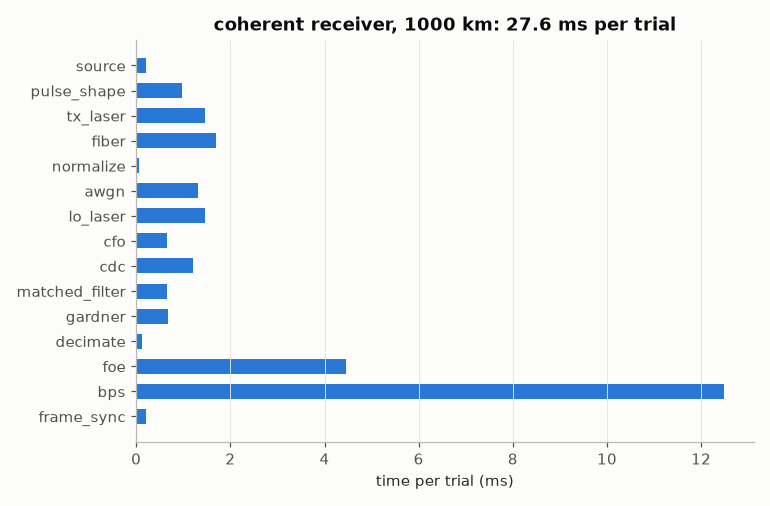
        source     0.210 ms    0.8 %
   pulse_shape     0.969 ms    3.5 %
      tx_laser     1.454 ms    5.3 %
         fiber     1.693 ms    6.1 %
     normalize     0.068 ms    0.2 %
          awgn     1.307 ms    4.7 %
      lo_laser     1.457 ms    5.3 %
           cfo     0.663 ms    2.4 %
           cdc     1.212 ms    4.4 %
matched_filter     0.652 ms    2.4 %
       gardner     0.684 ms    2.5 %
      decimate     0.123 ms    0.4 %
           foe     4.448 ms   16.1 %
           bps    12.488 ms   45.2 %
    frame_sync     0.210 ms    0.8 %
          link    27.646 ms  100.0 %

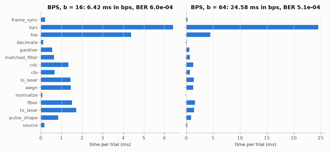
Comparing settings. Blind phase search tests b phases over a window of 2n + 1 symbols: its cost grows with both. The profile of two settings side by side shows what the finer search costs, and the error rate what it buys.

variants = {
    "BPS, b = 16": link.replace(bps=B.Bps(n=32, b=16)),
    "BPS, b = 64": link.replace(bps=B.Bps(n=32, b=64)),
}
fig, axes = plt.subplots(1, 2, figsize=(10, 4.6), sharey=True)
for ax, (name, chain) in zip(axes, variants.items(), strict=True):
    res = chain.run(
        grid={"length_km": [1000], "snr_db": [18]},
        metrics={"report": ["ber"], "skip_start": 2560, "skip_end": 256},
        stop={"max_trials": 16},
        profile=True,
    )
    rows = res.profile()
    bps = next(r for r in rows if r["block"] == "bps")
    bars(
        rows,
        ax,
        f"{name}: {bps['time_ms']:.2f} ms in bps, BER {res[0]['metrics']['ber']['value']:.1e}",
    )
fig.tight_layout()

The price of a Python block. The matched filter written with NumPy, with the same taps as the native block (comnum.pulse_shape()), inserted in place of it. A chain with a Python block runs on the Python runner, which times the native blocks too, so the two matched filters are measured the same way, one trial at a time.

taps = comnum.pulse_shape("rrc", 2, n_taps=1025, rolloff=0.2)


def numpy_matched_filter(frame, rng):
    frame.samples = np.convolve(frame.samples, taps, mode="same")


python_link = link.replace(matched_filter=numpy_matched_filter)
campaign = {
    "grid": {"length_km": [1000], "snr_db": [18]},
    "metrics": {"report": ["ber"], "skip_start": 2560, "skip_end": 256},
    "stop": {"max_trials": 8},
    "profile": True,
}
native = link.insert_after("source", noop=lambda f, r: None).run(**campaign).profile()
python = python_link.run(**campaign).profile()
for name, rows in [("native", native), ("NumPy", python)]:
    r = next(r for r in rows if r["block"] == "matched_filter")
    print(f"matched filter, {name:>6}: {r['time_ms']:.3f} ms per trial")

matched filter, native: 0.397 ms per trial
matched filter,  NumPy: 6.599 ms per trial

From the command line. comnum run specs/coherent_link.yaml --profile (or profile: true in the file) prints the same table after the results, averaged over the conditions, and the JSON and CSV reports carry the <block>.time_ms metrics of every condition:

profile: mean time per trial over 12 conditions
                  source       0.312 ms    1.4 %
             pulse_shape       0.901 ms    4.1 %
                     ...
                    link      22.004 ms  100.0 %

Two cautions. The first trial of a condition pays the allocations of the blocks, so profile with a few trials rather than one; and a block that draws (a source, a channel) is timed with its random draws, which the parallel runner shares between trials no differently.